Home
Tutorials
Tutorials show you how to use Simcenter STAR-CCM+ for various applications in a step-by-step format with recommendations for setup, initialization and steps of the solution process specific to the application. Macro and simulation files are available for download for a large proportion of cases.
Aeroacoustics
The tutorials in this set illustrate various Simcenter STAR-CCM+ features for solving aeroacoustic simulations.
Signal Post-Processing: FFT and Wavenumber
Several further analyses are possible using the simulation history file from the earlier tutorial, DES and FW-H On-The-Fly: Noise from a Cylinder (Unsteady Analysis). These analyses are covered in this tutorial.
Visualizing the Sound Pressure Level at Different Frequencies
The solution history file can be used in a fast Fourier transform to visualize the sound pressure level on the stored surfaces at selected frequencies.

Share

Link: copied

Breadcrumb: copied

Tutorials
Tutorials show you how to use Simcenter STAR-CCM+ for various applications in a step-by-step format with recommendations for setup, initialization and steps of the solution process specific to the application. Macro and simulation files are available for download for a large proportion of cases.
- Using Tutorial Macros and Files
  Macros, input files, and final simulation files for a range of tutorials are provided as an optional download package on the Support Center website. These macros and final simulation files are provided as an aid to the written tutorials, so that you can check your final results against the downloaded files, or against a simulation that is built and run using the macros.
- Introduction
  Welcome to the Simcenter STAR-CCM+ introductory tutorial. In this tutorial, you explore the important concepts and workflow. Complete this tutorial before attempting any others.
- Foundation Tutorials
  The foundation tutorials showcase the major features of Simcenter STAR-CCM+ in a series of short tutorials.
- Geometry
  The tutorials in this set illustrate various Simcenter STAR-CCM+ features for creating and working with parts and 3D-CAD.
- Mesh
  The tutorials in this set illustrate various STAR-CCM+ features for building CFD meshes.
- Incompressible Flow
  The tutorials in this set illustrate various Simcenter STAR-CCM+ features for incompressible fluid flows as well as porosity and solution recording
- Compressible Flow
  The tutorials in this set illustrate various Simcenter STAR-CCM+ features for compressible fluid flows as well as harmonic balance.
- Heat Transfer and Radiation
  The tutorials in this set illustrate various Simcenter STAR-CCM+ features for heat transfer, radiation, and thermal comfort.
- Multiphase Flow
  The tutorials in this set illustrate various Simcenter STAR-CCM+ features for simulating multiphase fluid flow problems
- Discrete Element Method
  The tutorials in this set illustrate various Simcenter STAR-CCM+ features for simulating Discrete Element Method problems
- Motion
  The tutorials in this set illustrate various STAR-CCM+ features for simulating problems with moving geometries and meshes, dynamic fluid body interaction, and rigid body motion:
- Reacting Flow
  The tutorials in this set illustrate various Simcenter STAR-CCM+ features for simulating reacting flows such as combustion.
- Solid Stress
  The tutorials in this set illustrate various Simcenter STAR-CCM+ features for computing deformation, strain, and stresses in solid regions. They also show how such computations can be coupled to the fluid behavior in an analysis of fluid-structure interaction.
- Aeroacoustics
  The tutorials in this set illustrate various Simcenter STAR-CCM+ features for solving aeroacoustic simulations.
  - Broadband Models: Noise from a Cylinder (Preparation)
    This tutorial demonstrates how to set up aeroacoustics problems in Simcenter STAR-CCM+. The flow around a cylinder is used in the simulation to describe the required steps.
  - DES and FW-H On-The-Fly: Noise from a Cylinder (Unsteady Analysis)
    In the previous section of this tutorial, you completed the steady-state analysis runs for qualifying the volume mesh. In this section, continuing from the previous simulation file, you set up the final transient run for an unsteady analysis of the near field and an FW-H analysis of the far field.
  - Ffowcs Williams-Hawkings: Sound Propagation
    This tutorial compares the Post FW-H model with the FW-H On-The-Fly model.
  - Signal Post-Processing: FFT and Wavenumber
    Several further analyses are possible using the simulation history file from the earlier tutorial, DES and FW-H On-The-Fly: Noise from a Cylinder (Unsteady Analysis). These analyses are covered in this tutorial.
    - Loading the Initial Simulation
      You start from existing simulation and solution history files that contains objects and solution data from the tutorial DES and FW-H On-The-Fly: Noise from a Cylinder (Unsteady Analysis).
    - Visualizing the Pressure at Different Time-Steps
      You set up a scalar scene to view the pressure on the cylinder wall and on the plane section. To retrieve the pressure at different time-steps from the simulation history file, you use the solution view cylinderPressureData.
    - Visualizing the Sound Pressure Level at Different Frequencies
      The solution history file can be used in a fast Fourier transform to visualize the sound pressure level on the stored surfaces at selected frequencies.
    - Determining the Group Velocity of the Disturbances
      A wavenumber-frequency diagram (or fk plot) is used to determine the group velocity at which disturbances propagate along the domain.
    - Summary
      This tutorial covered post-processing for spectral and wavenumber analysis.
  - Acoustic Wave Modeling: Noise from a Cylinder
    This tutorial demonstrates how to set up an acoustic wave simulation in Simcenter STAR-CCM+. The flow around a cylinder is used in the simulation to describe the required steps.
  - Lighthill Wave and Perturbed Convective Wave Modeling: Simplified HVAC Duct
    Noise generated by the air handling components in heating, ventilation, and air conditioning (HVAC) systems is a large contributor to interior cabin sound levels. Investigating the sources of noise and modifying the design accordingly, leads to better and quieter systems.
  - Sponge Layer Modeling: Simplified Tailpipe
    Unsteady aeroacoustics simulations require effective non-reflective boundary conditions to prevent spurious reflected acoustic waves from the boundaries of the computational domain interfering with the aeroacoustic results.
- Electromagnetism
  The following tutorials illustrate features for solving problems that involve electromagnetic fields.
- Electrochemistry
  The following tutorial demonstrates chemical reactions induced by an electrical current.
- Battery
  The tutorials in this set illustrate various Simcenter STAR-CCM+ features for setting up a battery model:
- Automation
  The tutorials in this set illustrate various Simcenter STAR-CCM+ automation and macro features.
- Design Exploration
  The tutorials in this set illustrate various features for running design exploration studies in Design Manager.
- Coupling with CAE Codes
  The tutorials in this set illustrate various Simcenter STAR-CCM+ features for coupling with CAE codes:
- Analysis Methods
  The tutorials in this set illustrate various Simcenter STAR-CCM+ features for analysing and visualizing simulation data.
- Simcenter STAR-CCM+ In-cylinder
  The tutorials in this set illustrate features for simulating internal combustion engines in Simcenter STAR-CCM+ using the dedicated add-on Simcenter STAR-CCM+ In-cylinder.

Visualizing the Sound Pressure Level at Different Frequencies

The solution history file can be used in a fast Fourier transform to visualize the sound pressure level on the stored surfaces at selected frequencies.

To visualize the sound pressure level at different frequencies:

Right-click the Tools > Data Set Functions node and select New > Surface Time History (h[s]).
Select the h(s) 1 node and set the following properties:

Property Setting

Start Signal 0.02 s

End Signal 0.0533 s
Right-click the h(s) 1 > Imported node and select New derived data from surface.

Select the Multi-Point Time History node and set the following properties:


Property	Setting
Representation	cylinderPressureData
Data Surfaces 1	Regions > Body 1 > Boundaries > Cylinderwall Derived Parts > Plane Section
Target Surfaces	Regions > Body 1 > Boundaries > Cylinderwall Derived Parts > Plane Section
Field Function 1	Pressure
Update Active	Enabled

Right-click the Data Set Functions node and select New > Surface Time Fourier Transform (G[h[s]]).

Select the G(s) 1 node and set the following properties:


Property	Setting
Analysis Blocks	2
Overlap Factor	0.5
Start Signal	0.02 s
End Signal	0.0533 s
Window Function	Hann

Right-click the G(s) 1 > Imported node and select New derived data from derived data.

Expand the Multi-Point FFT node and set the following properties:


Node	Property	Setting
Multi-Point FFT	Input Time History	Multi-Point Time History
Multi-Point FFT	Update Active	Activated
Output Control	Frequency Mode	Frequency
Output Control	Output Field	Sound Pressure Level
Display slider control	Slider Value	500

Create a scalar scene, rename it to Sound Pressure Level, and set the following properties:


Node	Property	Setting
Sound Pressure Level
Outline 1
Parts	Parts	Parts > Body 1
Scalar 1	Contour Style	Smooth Filled
Parts	Parts	Derived Data > Multi-Point FFT
Scalar Field	Function	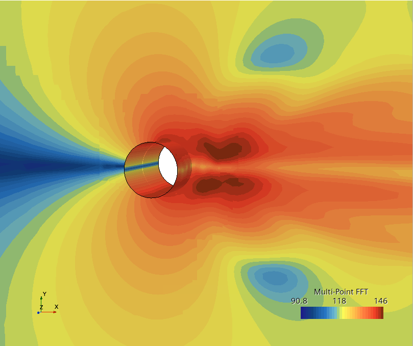Derived Data > Multi-Point FFT

The SPL (dB) values at the top and bottom of the cylinder exactly match the point spectra dB levels at 500 Hz.

To view the sound pressure level at a different frequency, select the Multi-Point FFT > Display slider control node and set Slider Value to the frequency of interest.
Save the simulation.