Applying Blade Parametric Coordinates
When defined correctly, a blade parameterization registers field functions that you can use in creating profile derived parts on which you can plot quantities such as pressure (for blade loading). By applying the Leading-Trailing function, you can create an unwrapped plot showing suction and pressure sides of the blade in succession.
-
Right-click the Derived Parts node and select .
Although an isosurface is used here, the result is a line (profile) rather than a 2D surface.
- In the Create Isosurface panel (assuming that you have a scene open), set the following properties:
Property Value Input Parts Select the part surface for the pressure side of the blade. Scalar [blade parameterization] Root-Tip Extraction Mode Single Value Isovalue Set this value according the the location across the blade on which you want to see blade loading. For example, 0.5. - Click Create.
-
Repeat the previous step, but this time create an isosurface for the suction side of the blade. Scalar, Extraction Mode, and Isovalue should be the same as for the first isosurface.
You can use the same isosurface for both sides of the blade if you prefer. The choice depends on whether you want to distinguish visually between the suction side and the pressure side.
- Right-click the Plots node and select .
-
Edit the [xy plot] node and set the following properties:
Node Property Value [xy plot] Parts Choose both derived parts from the steps above (isosurface profiles based on [blade parameterization] Root-Tip).  X Type
Data Type Scalar  Scalar Function
Field Function [blade parameterization] Leading-Trailing Observe that the field function here is not the Root-Tip function, but Leading-Trailing. This choice gives the unwrapped plot across both blade surfaces.
 Scalar Function
Field Function Absolute Pressure (for blade loading — you can choose other scalars as required).
[isosurface for pressure side]Sort Plot Data Activated (This property is not activated by default — but activating it is necessary for achieving the correct plot.)
[isosurface for suction side]An example of the resulting plot is as follows: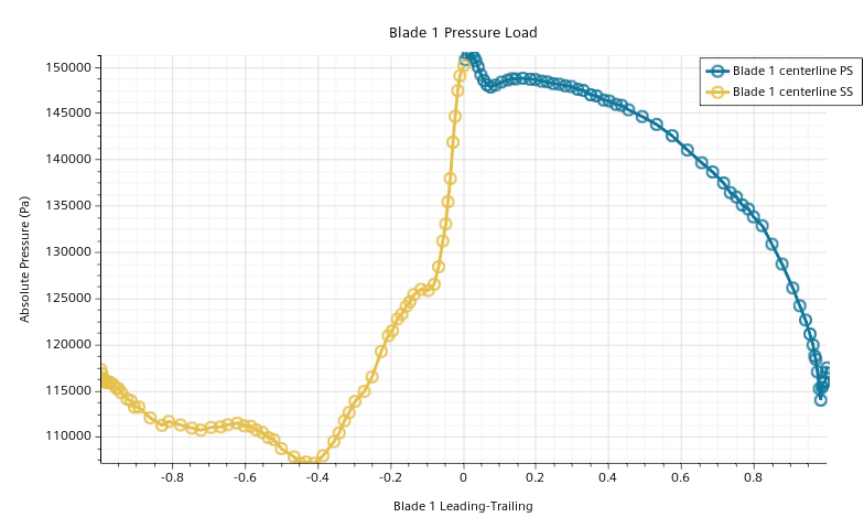
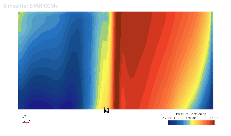
When you apply the blade embedding transform on a displayer, Simcenter STAR-CCM+ unwraps both sides of the blade in a single 2D image.
- To obtain an unwrapped image of the blade surfaces:
- Create a scalar scene.
- Select the node and set Parts to include both pressure and suction sides of the blade.
- Set Scalar Field to an appropriate quantity, for example, Pressure.
- Select the [scalar displayer] node and set Transform to Embedding: [blade parameterization] (for example, Embedding: Blade 1).
A 2D unwrapped image of the scalar quantity is shown.