Coordinate System Averaging

In Simcenter STAR-CCM+, the csavg() function allows you to average data along any direction of a specified coordinate system. Coordinate system averaging provides a two-dimensional meridional view for the three-dimensional solution. While the meridional view is commonly used in turbomachinery, it is generally suitable for applications that involve axisymmetric regions.

Given a field function $ϕ$ , Simcenter STAR-CCM+ calculates the average of $ϕ$ along a direction $θ$ as:

Figure 1. EQUATION_DISPLAY

\bar{ϕ_{θ}} = \frac{\int_{θ_{1}}^{θ_{2}} ϕ \partial θ}{\int_{θ_{1}}^{θ_{2}} \partial θ} = \frac{1}{(θ_{2} - θ_{1})} \int_{θ_{1}}^{θ_{2}} ϕ \partial θ

(13)

The field function is integrated along isolines on a slice to obtain a two-dimensional grid of averaged values. The number of isolines on a slice is determined by the number of integration lines. The grids obtained are interpolated to sweep through the domain in the slicing direction.

To calculate the average of a field function using the csavg() function, you use the following syntax:

csavg(value, @CoordinateSystem("Laboratory"), averagingDirection, sliceDirection, numSlices, integrationsPerSlice)

where:

value is the field function being averaged (both scalars and vectors can be averaged)
CoordinateSystem("Laboratory") is the coordinate system in use for the averaging
averagingDirection is the averaging direction
sliceDirection is the slice direction
numSlices is the number of slices
integrationsPerSlice is the number of integration lines per slice

The csavg() function does not support non-contiguous regions.

For example, to obtain the circumferentially averaged axial velocity in a user-defined cylindrical coordinate system, you can create a user-defined field function with the following expression:

csavg(${AxialVelocity}, @CoordinateSystem("Labratory.Cylindrical 1"), 1, 0, 50, 60)

In this example, the slices are taken radially.

Note	When defining the direction in cylindrical coordinates, 0 corresponds to the radial axis (along r), 1 corresponds to the circumferential axis (along theta), and z corresponds to the longitudinal axis (along z).

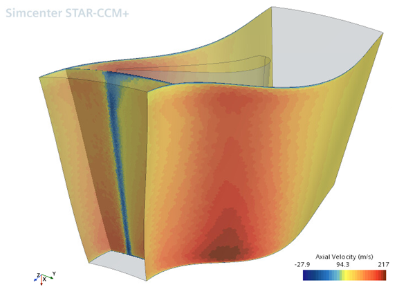
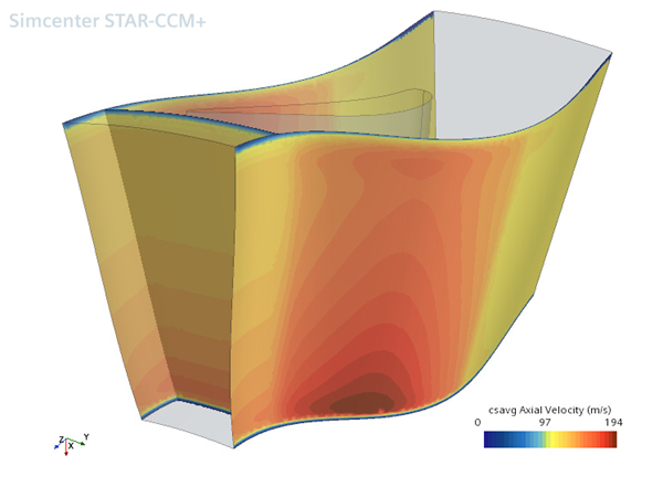
The following example evaluates the axial velocites in a turbine stage, as determined by the function definition above. This is an illustrative example; to obtain 2D average views and 1D average surface plots for turbomachinary cases in Simcenter STAR-CCM+, it is recommended you create an average profile derived part. See Defining an Average Profile (Turbomachinery).

The first scalar scene illustrates the axial velocities at the trailing edge of a turbine blade on an isosurface at constant z:

The second scalar scene illustrates the circumferentially averaged axial velocities, as defined by the csavg() function above:

The axial velocity plot illustrates the averaged axial velocity values (yellow dots) obtained from a distribution of axial velocities (blue dots) on the constant z isosurface at the trailing edge of the blade.

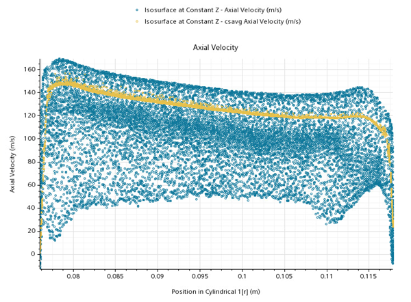
A similar plot can be obtained by creating a 1D average profile. See Defining an Average Profile (Turbomachinery)

The following examples are from a rotor case.

This scalar scene illustrates projection of vertices to the grid:

The blue-gray plane shows a constant z slice.
Black lines are averaging lines of constant r.
The results from multiple slices appear in a two-dimensional average mesh.

The following image shows these values in a plot:

Red dots are the resulting average mesh.
Blue “x” symbols are the (z, r) vertices from the region projected onto this mesh.
Green dots are extrapolated (halo) nodes from the average mesh.

For comparison, look at the scalar-scene representation of the average mesh.

The scalar scene in the following screenshot shows the rotor case using the following user-defined field function:

csavg($AbsoluteTotalPressure, @CoordinateSystem("Cylindrical 1"), 1, 2, 20, 60)

This field function takes the average of Absolute Total Pressure, using the Cylindrical 1 coordinate system in the $θ$ direction, and slicing in the z direction. It uses a 20 x 60 averaging mesh -- that is, this mesh has 20 z-slices and, for each z-slice, 60 averaging lines (or r-slices).