Defining an Average Profile (Turbomachinery)

In Simcenter STAR-CCM+, the average profile part evaluates the averages of fields from the input surfaces into discrete bins using the parameters that the axisymmetric parameterization computes. It provides a projected profile of circumferentially-averaged values based on the field values of the input surfaces of revolution (such as isosurfaces and plane sections). This derived part is typically used for post-processing results of a turbomachinery analysis.

Although any surface-type part can be selected as an input for an average profile part, to generate a valid average profile geometry, the input surface must be a surface of revolution around the z-axis of the cylindrical coordinate system used in the parameterization. This is reflected in the tooltip of the input parts.

Like other derived parts, you can post-process averaged fields on the average profile part in a scene, plot, report, or table. Field values are averaged in each bin using the area weighting method. However, consider the following:

  • Geometric quantities such as Position and its components represents the spatial location of the average profile geometry, thus they are not averaged fields.
  • To ensure consistency between the vertex values and face center values of certain fields such as Wall Distance, use smoothing where applicable:
    • Smooth Filled in scalar scenes
    • Smooth Values in plots and reports
    • Data on Vertices in tables

The following procedure assumes that you already have an axisymmetric parameterization defined in your simulation:

  1. Follow the general procedure outlined in the section, Defining Derived Parts General Workflow. Choose the menu option, New Part > Average Profile.
  2. Specify the input parts and display option as described in the section, Defining Derived Parts General Workflow.
  3. Complete the average surface definition by specifying the following properties:
    1. Parameterization: Select a parameterization. See Parameterization of Volume of Revolution.
    2. Binning Mode: Set this property to either of the following:
      • Equal distance - creates equally spaced bins according to the number that you specify. In the node properties, this number is the Resolution property of the Equal Distance child node. In the dialog, the property appears as Binning Resolution.

        The following example demonstrates the effect of the different Resolution on an average profile:

        Resolution Average Profile
        2

        15

        30

      • Mesh resolved: defines the number of bins automatically to half the local mesh size. This option can provide sufficiently accurate results without requiring you to manually set the size. In addition, it works better for non-homogenous meshes as it adapts to the local mesh size. An example is shown below:


    3. Functions: Select a field function with which to map back to the input surfaces.

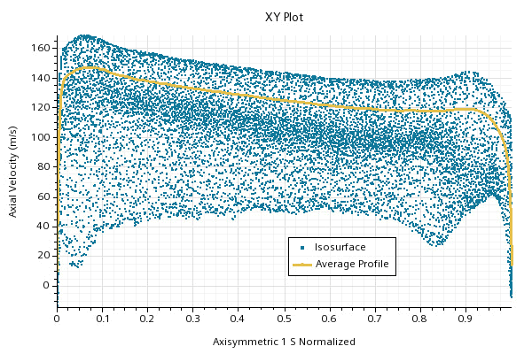
      When you select an existing field function, for example Axial Velocity, for this property, a new field function appears, Average Profile: Axial Velocity. The circumferentially averaged field can be displayed on a 2D surface in the same shape as the input surface in order to examine it in context with the 3D model.

    4. Weighting Mode: To determine whether you use a weighted average, set this property to one of the following:
      • Area
      • Area-Adjusted Scalar Function
      • Mass Flow

      When using Area-Adjusted Scalar Function, you specify the scalar function by selecting it in the Weight function property of the Weight function sub-node of the derived part node, or in the Weight function property of the in-place dialog.

      NoteAn Average Profile field function, which is created when a selection is made in the Functions property of the Average Profile node, cannot be selected for the Weight function property as this creates circular dependency.
    For more information on the available properties, refer to the section Average Profile Properties.

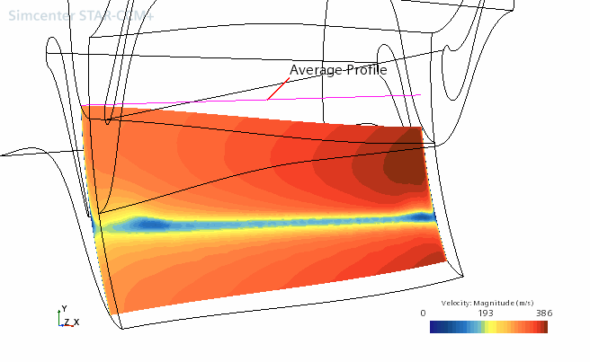
    This derived part appears as a simple line in the scene because the 2D surface has been averaged to a 1D profile. It shows that it is consistent with the surface input.


    The averaged data can be viewed in an XY plot.