Field Histories Example: Pressure-Time Derivatives
Field histories provide, among other uses, the ability to compute time derivatives of solution quantities. However, you must correctly account for any motion in the field.
Examples of applications include:
- Using a pressure derivative to investigate acoustics
- Using momentum time derivatives to detect sources of fatigue through fluctuations in force/moment
- Using turbulent kinetic energy time derivatives to identify power fluctuations
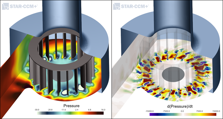
Pressure-Time Derivative in a Squirrel Cage Blower
In the illustration below for a squirrel cage blower, pressure contours are shown on the left and (second order error, backward difference formulation) is shown on the right. This data was created using field functions that leverage field history stored results.
- History of Position:
- Sliding Sample Window Size: 2
- Field Function: Position
- Trigger: Time Step
- Resulting field function names: History of Position Sample 0, History of Position Sample 1
- History of Pressure:
- Sliding Sample Window Size: 2 or more (depending on stencil width)
- Field Function: Pressure
- Trigger: Time Step
- Resulting field function names: History of Pressure Sample 0, History of Pressure Sample 1, and so on
From basic transport equations, the substantial or material derivative for pressure is:
Hence to obtain the pressure derivative in a simulation with mesh motion, you must evaluate:
The mesh velocity in each cell can be
obtained using a field history that samples Position, and for
which the resulting field functions are HistoryofPositionSample0
(current time-step) and HistoryofPositionSample1 (previous
time-step). These are combined in a field function MeshVelocity
as:
MeshVelocity = ($${HistoryofPositionSample0}-$${HistoryofPositionSample1})/${dt}where dt is another
field function that contains the time-step. This function can be supplied as a
scalar parameter.
The velocity-gradient term can be
computed by a field function, Pconvective_current:
Pconvective_current = dot($${MeshVelocity},grad(${Pressure}))Where Pressure is the
built-in solution field function.
For computing the final pressure derivative, the simplest first order computation using field functions from the field history of pressure is:
(${HistoryofPressureSample0}-${HistoryofPressureSample1})/(1.0*${dt}) - ${Pconvective_current}A more complex expression, with a wider stencil (and requiring a Sliding Sample Window Size of 3 for Pressure), is:
(3.0*${HistoryofPressureSample0}-4.0*${HistoryofPressureSample1}+${HistoryofPressureSample2})/(2.0*${dt}) - ${Pconvective_current}Using time derivative expressions with higher order accuracy can help to reduce the noise, but at the cost of an increased size for the simulation file.
If your simulation has no motion, then
Pconvective_current is not required.