Post-Processing Harmonic Balance Solution Data
Harmonic Balance offers the ability to visualize a flow variable either in the time domain (for example, at specific time instants) or in the frequency domain (for example, the Real component of the second Fourier mode).
-
For every blade row, the solution can be reconstructed and visualized in one or more blade passages, and not just in the modeled blade passage.
- The solution can be reconstructed and plotted at any instant of time.
- The solution views can be easily switched between time domain and frequency domain visualization. This can be helpful for understanding the unsteady flow features.
You can examine and analyze the results of a harmonic balance simulation on two different representations. When you visualize field functions that represent unsteady or time-varying quantities in a scene, report, or plot, the Representation determines the meaning of the displayed solution field. The choice of representation does not influence the meaning of time-invariant quantities. You can choose between the following representations:
- Volume Mesh—displays the time-mean solution field.
- HB Solution View—displays the state of the solution as selected in the corresponding HB Solution View node, such as physical time, Fourier mode, time-level, or filtered mode.
To visualize Harmonic Balance solution data:
- Create a scalar or a vector scene and select a field function, for example, Temperature.
-
Select the node. By default,
Representation is set to
Volume Mesh.
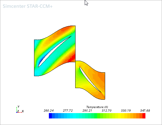
The following screenshot shows the time-mean temperature solution on two meshed blade rows, both displaying only the modeled blade passage. This time-mean temperature is displayed on the Volume Mesh representation.
If you have visualized the variable as part of a steady-state simulation on the blade row geometry, now you can activate the Harmonic Balance model and still retain the visualization.
-
To visualize the Harmonic Balance solution in different modes and on multiple
blade passages, create an HB Solution View:
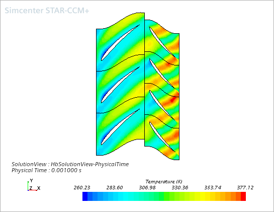
The following screenshot shows the temperature at a physical time of 0.001 s on three blade passages for the first blade row and four blade passages for the second blade row.
-
To visualize a field function in a different mode or on a different number of
blade passages, you can create additional HB Solution Views.
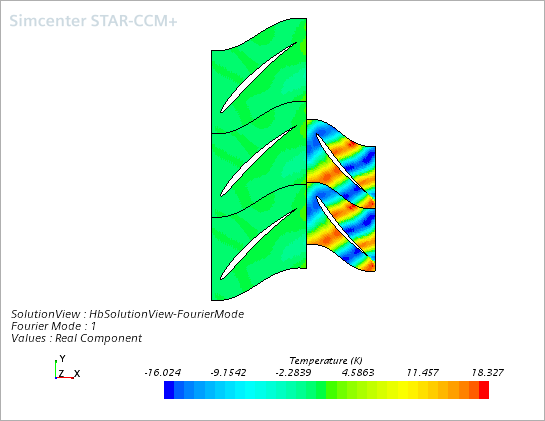
For example, using the following settings in another HB Solution View:results in the following temperature distribution.
Node Property Setting HB Solution View 2 Mode Fourier Mode  Fourier
Mode
Fourier
ModeMode 1 Output Option Real Blade
Rows Blade Row
1
Blade Row
1Blade Passage Selection [-1,1] Blade Row 2Blade Passage Selection [0,1] Rename the HB Solution View 2 node to HBSolutionView-FourierMode, then drag-and-drop it to the graphics window to display the Fourier mode temperature scene.