Plotting Graphs
Plot the lift and drag coefficients to determine when the analysis has converged.
-
Right-click the Reports node and select .
A new report node named Force Coefficient 1 is created.
-
Rename this node
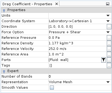
Drag Coefficient then enter the following information:
Property Value Units Empty Coordinate System Direction [1.0, 0.0, 0.0] Force Option Pressure + Shear Reference Pressure 0.0 Pa Reference Density 1.177 kg/m^3 Reference Velocity 252.0 m/s Reference Area 1.0 m^2 Parts [Fluid: wall] Number of Bands 0 Representation Volume Mesh Smooth Values Deactivated 
- Right-click the Drag Coefficient node and select Create Monitor and Plot from Report.
A new plot node appears named Drag Coefficient Monitor Plot.
- Select the Drag Coefficient Monitor Plot node and set the Title to Drag Coefficient Monitor Plot.
To create a plot for the lift coefficient:
- Repeat the steps described above to create and display a plot for the lift coefficient. All settings are the same as for the drag coefficient.
- Rename the report node Lift Coefficient and set its Direction property to [0.0, 1.0, 0.0].
- Select the Lift Coefficient Monitor Plot node and set the Title to Lift Coefficient Monitor Plot.
Experimental data for the pressure coefficient on the airfoil are provided in file aero_exp.xy in the doc/startutorialsdata/compressibleFlow/data directory. Plot the data on a graph alongside the results of the analysis.
To plot the experimental data:
- Right-click the node and select .
- Set Files of type: to (*.xy), then locate and open the file aero_exp.xy.
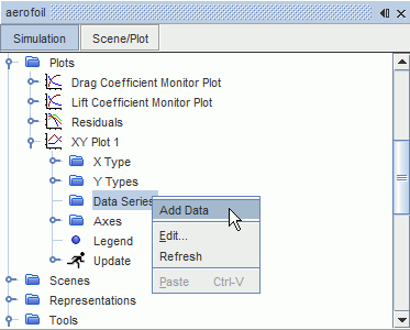
- Right-click the Plots node and select .
-
Right-click the
node and select
Add Data.

- In the Add Data Providers to Plot window, select aero_exp.
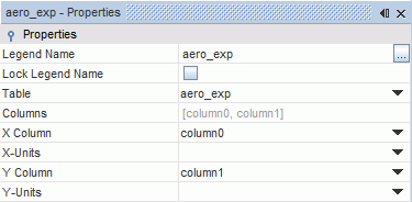
- Select the node and set aero_exp for the Table property.

A graph of the experimental data appears in XY Plot 1.
To add the numerical data to the same graph:
- Select the XY Plot 1 node and click the Parts property.
- Select Fluid: wall in the XY Plot 1 - Parts dialog.
- Select the node and set Pressure Coefficient for the Field Function property.
The initial pressure coefficient is shown in the XY Plot 1 as being zero everywhere.
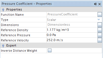
The pressure coefficient requires specification of a reference pressure and a reference velocity.
-
Select the node and enter a Reference Density of
1.177 kg/m^3 and a Reference
Velocity of 252 m/s, have the settings shown
below:

The usual convention in aerodynamics problems is to reverse the y-axis orientation in pressure coefficient plots.
-
Select the
node and set the following properties:
Property Setting Preferred X-Axis Left Axis Preferred Y-Axis Bottom Axis - Select the and activate Reverse.
-
To set the correct titles for the plot:
- Select the node and set Title to Pressure Coefficient Comparison.
- Within , select the node and set Title to Distance (m).
- Select the node and set Title to Pressure Coefficient.
- Save the simulation.