Finite Element Solid Energy Model Reference

The Finite Element Solid Energy model is compatible with solid and shell regions (see Finite Element Solid Shells Heat Transfer). Shell regions require conformal internal interfaces for the shared edges between shell parts. Hub interfaces, internal (boundary-based) and mapped contact interfaces are not supported (see Interface Type). For shell regions, you can use either the Quadrilateral or Triangular volume meshers.


Theory	See Energy Equation in Solids.
Provided By	[physics continuum] > Models > Optional Models
Example Node Path	Continua > [Solid Physics Continuum] > Models > Finite Element Solid Energy
Requires	Physics Models: Space: Three Dimensional Material: Solid or Multi-Part Solid
Compatible Meshers	Directed Mesher Tetrahedral Mesher Thin Mesher For meshing guidelines, see Mesh Requirements and Guidelines.
Activates	Material Properties	Density Specific Heat Thermal Conductivity See Material Properties.
	Initial Conditions	Static Temperature. See Initial Conditions.
	Boundary Inputs	`Thermal Specification` . See Boundary Inputs.
	Region Inputs	`Energy Source Option` `Lumped Heat Capacity Matrix Option` `Mid-Side Vertex Option` See Region Inputs.
	Interface Inputs	`Energy Coupling Option` (for fluid/solid interfaces of type Mapped Contact Interface). See Interface Inputs.
	Monitors	Temperature Thermal Load Thermal Potential See Monitors.
	Solvers	Finite Element Solid Energy (uses either the Sparse Direct Solver or the Iterative solver) See Solver Settings.
	Field Functions	Boundary Heat Flux, Heat Flux, Specific Heat, Temperature, Temperature Gradient, Temperature Time Derivative, Thermal Conductivity. See Field Functions.

Material Properties

Currently, you can define the thermal properties of the solid material using constant values. You cannot define the thermal properties as functions of the solid temperature.

Density

Defines the mass per unit volume in the undeformed state (

ρ

in Eqn. (1660)). When using the Finite Element Solid Energy model in combination with Solid Stress model, this is the solid density in the undeformed state.

Specific Heat

Defines the specific heat of the solid material (

C_{p}

in Eqn. (1660)) as a constant profile. The specific heat specifies the heat per unit mass that is required to increase the solid temperature by 1 °C.

Thermal Conductivity

Defines the thermal conductivity of the solid material (

k

in Eqn. (1661)). The available methods are:

Method	Corresponding Value Nodes
Constant, Field Function, Polynomial in T, Table(T) Suitable for isotropic materials.	Thermal Conductivity > Constant, Field Function Specify $k$ as a scalar using either a constant value, a field function, a polynomial function of temperature, or a table of temperature values.
Anisotropic, Orthotropic, Transverse Isotropic Suitable for non-isotropic materials.	Thermal Conductivity > Anisotropic, Orthotropic, Transverse Isotropic Specify $k$ as a second-order tensor (see Tensor Quantities). [Region] > Physics Values > Thermal Conductivity Orientation Specifies the local orientation of the tensor. For more information, see Orientation Manager and Local Orientations.

When the thermal conductivity is a function of temperature, the discretized energy equation contains non-symmetric terms. In this case, Simcenter STAR-CCM+ neglects the non-symmetric terms in the linearization (modified Newton approach).

Initial Conditions

Static Temperature: Allows you to initialize the solid temperature to a specified scalar profile.

Boundary Inputs

Available for solid and shell wall boundaries. Unlike the Solid Stress model, the Finite Element Solid Energy model does not require segments.

Thermal Specification

Specifies the method that Simcenter STAR-CCM+ uses to define the thermal behavior at the solid boundaries.

Method	Activated Values and Conditions
Adiabatic No energy transfer occurs at the boundary.	None
Heat Flux Allows you to specify the heat flux across the boundary (see ${\dot{q}}^{"}$ in Eqn. (1660)).	Heat Flux Boundary-normal heat flux entered as a scalar profile. Specify a negative value for heat leaving the boundary, or a positive value for incoming heat.
Heat Source Allows you to specify the total heat at the boundary.	Heat Source Total heat entered as a scalar profile.
Temperature Allows you to specify the temperature at the boundary.	Static Temperature Boundary temperature entered as a scalar profile.
Convection Allows you to specify the convection flux across the boundary (see Eqn. (1661)).	Ambient Temperature Reference temperature ( $T_{r e f}$ in Eqn. (1661)), entered as a scalar profile. Heat Transfer Coefficient Heat transfer coefficient ( $h$ in Eqn. (1661)), entered as a scalar profile.

When modeling conjugate heat transfer between a fluid and a solid, Simcenter STAR-CCM+ automatically sets the thermal specification of the boundaries at the two sides of the fluid-structure interface. See Interface Inputs.

Time Averaging Option

Available at fluid-structure interface boundaries. At an interface boundary, this option allows you to specify whether the thermal fields (that is, the temperature coming from the solid boundary and the convective flux coming from the fluid boundary) are time-averaged before they are mapped to the other side of the interface. For more information, see Time Averaging Option.

Region Inputs

Energy Source Option

Allows you to define an additional source of energy for the solid region. You can use this option to account for the thermal energy coming from phenomena that are not explicitly modeled in the simulation.

Each of the following methods, except for None, activates a physics value with the same name where you specify the source.

None—no energy source is added.
Volumetric Heat Source—defines a heat source per unit volume (W/m³) as a scalar profile.
Total Heat Source—defines a heat source (W) as a scalar profile.
Specific Heat Source—defines the specific heat (W/kg) as a scalar profile.

Lumped Heat Capacity Matrix Option

Lumping the heat capacity matrix is a technique that reduces unwanted oscillations in the numerical solution of the energy equation Eqn. (1660). These spurious oscillations, which are expected in finite element formulations of the energy equation, typically occur in regions in which the thermal boundary layer is thin and cannot be captured by the specified spatio-temporal discretization.

This generally occurs when:

Figure 1. EQUATION_DISPLAY

\frac{α Δ t}{Δ x^{2}} < 1

(348)

where $α$ is the thermal diffusivity of the material, $Δ x$ is the average mesh element size, and $Δ t$ is the simulation time-step.

Activating lumping is recommended in regions that satisfy Eqn. (348). Lumping is only available for meshes that include first-order elements, that is, linear elements without mid-side nodes.

Mid-side Vertex Option

Allows you to remove or add mid-side vertices to the mesh. For more information, see Mid-side Vertex Option.

Interface Inputs

The Finite Element Solid Energy model is suitable for all interface topologies except Repeating interfaces.

Energy Coupling Option

Available for solid/fluid interfaces of type Mapped Contact Interface.

This option determines the method for coupling the thermal solutions at the fluid-structure interface (see Energy Coupling Option). When using the Finite Element Solid Energy model, Simcenter STAR-CCM+ automatically sets this option to Explicit. The explicit coupling option allows for automatic data exchange between non-conformal interface boundaries, without the need of using data mappers.

Energy Coupling Option	Conditions and Values at the Interface Boundaries
Explicit With explicit coupling, the solid temperature at the fluid convective flux are mapped across the two sides of the interface. Simcenter STAR-CCM+ automatically sets the solid interface boundary to use thermal field mapped from the fluid side of the interface.	Solid interface boundary: Ambient Temperature Heat Transfer Coefficient Set automatically based on the fields mapped from the fluid boundary. Fluid interface boundary: Static Temperature Set automatically based on the field mapped from the solid boundary. When using the explicit option, also set the `Time Averaging Option` physics condition at the fluid and solid interface boundaries. See Time Averaging Option.

Energy Coupling Option

Conditions and Values at the Interface Boundaries

Explicit: With explicit coupling, the solid temperature at the fluid convective flux are mapped across the two sides of the interface. Simcenter STAR-CCM+ automatically sets the solid interface boundary to use thermal field mapped from the fluid side of the interface.

Solid interface boundary:

Ambient Temperature
Heat Transfer Coefficient: Set automatically based on the fields mapped from the fluid boundary.

Fluid interface boundary:

Static Temperature: Set automatically based on the field mapped from the solid boundary.

When using the explicit option, also set the Time Averaging Option physics condition at the fluid and solid interface boundaries. See Time Averaging Option.

Constraint Mapping

Available for solid/solid interfaces of type Mapped Contact Interface.

Specifies the method that Simcenter STAR-CCM+ uses for constraining bonded surfaces. The available options are:

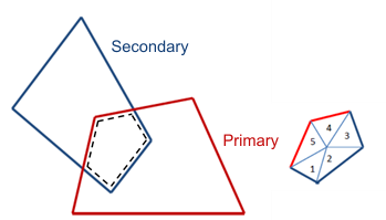
Node to Surface:
Default option. At the interface between two finite elements, a node on the secondary element is constrained to the nodes of the overlapping surface on the primary element. In general, this method requires low computational effort, although it does not conserve linear and angular momentum (in solid stress calculations) or heat flux (in solid energy calculations) and can lead to local inaccuracies in the computed stresses or temperature.
Surface to Surface:
At the interface between two finite elements, the overlapping surface of the secondary element with the primary element is subdivided in triangles. The constraints are satisfied in an integral or weak sense over the overlapping surface. Compared to the Node to Surface method, this method preserves linear and angular momentum (in solid stress calculations) or heat flux (in solid energy calculations), therefore increasing the accuracy of the computed stresses or temperature. However, this method requires more computational effort and the required memory increases with the number of cores in use.

This choice is only available for bonded mapped contact interfaces. Sliding interfaces automatically use the Node to Surface method.

For adjacent interfaces, which share perimeters and therefore vertices, you are advised to use the same constraint mapping method. Using both methods may result in over-constraining the shared vertices.

Monitors

Temperature: Solid temperature increment [K] (see Eqn. (4833)).
Thermal Load: Residual flux [W] (see Eqn. (4833)). The Thermal Load residual is equivalent to the Energy residual that is available for finite volume energy models. Both have the unit of power [W].
Thermal Potential: Thermal potential, defined with the unit of [WK] (see Eqn. (4838)). This monitor is available when you activate the Thermal potential property for the Finite Element Solid Energy Solver.

Finite Element Solid Energy Solver Properties and Controls

The available properties are:

Under-Relaxation Factor: The default value is 1. To speed up convergence and improve stability of the linear system, you can decrease the under-relaxation factor.
Temporary Storage Retained: When activated, the solver retains the temperature and thermal load residuals at the end of the iteration. You can access these residuals using the corresponding field functions.
Heuristic Resolution of Conflicting Constraints: When activated, Simcenter STAR-CCM+ uses a heuristic approach to resolve conflicting constraints and cyclic dependencies. In some cases, this resolution method can affect the solution and lead to unrealistic results. When this option is active, make sure that you assess the validity of the solution.
By default, this property is deactivated. In Simcenter STAR-CCM+ versions before 15.06, the heuristic conflict resolution was the default approach.

For common properties, see Common Properties.

Like the Solid Stress solver, the Finite Element Solid Energy solver has a control that allows you to choose the Integration Method. For more information on the available options, see Integration Method.

Field Functions

Boundary Heat Flux: Magnitude of the heat flux vector normal to the boundary.
Heat Flux: Heat flux vector ( ${\dot{q}}^{"}$ in Eqn. (1660)).
Specific Heat: Reflects the specific heat property specified for the solid material.
Temperature: Solid temperature, as computed by the Finite Element Solid Energy solver.
Temperature Gradient: Temperature gradient (see Eqn. (1661)).
Temperature Time Derivative: Derivative of the solid temperature with respect to time.
Thermal Conductivity: Reflects the thermal conductivity property specified for the solid material.