Preliminary Analysis
Before you begin the acoustic wave simulation, obtain a fully developed flow solution, then obtain mean flow pressure or velocity fields, according to the kind of simulation, and define filtering and damping.
-
For hybrid flow and aeroacoustics simulations with convection, set up a
Field Mean of Pressure monitor:
-
For aeroacoustic simulations using convective effects, set up
Field Mean monitors for the X, Y, and Z components of the velocity:
- Run the flow simulation to obtain the fully developed solution.
-
Activate the Acoustic Wave model and, under the Acoustic
Wave node, set the Mean Flow Pressure Reference property to
Specified.
This exposes the Mean Flow Pressure Reference and Mean Flow Velocity Reference child nodes.
-
To obtain the mean flow pressure field, set the
Mean Flow Pressure Reference to use the
Mean of Pressure field function.
-
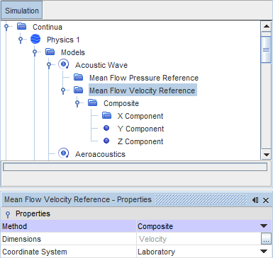
To obtain the mean flow velocity field, use one of the following procedures:
- Use the Composite method:
- Select the node and set the Method property to Composite.
- Expand the Composite node to expose the X Component, Y Component, and Z Component sub-nodes.
- In each sub-node, using the Method property, specify the value for each component of the velocity.
- Define a field function combining the individual mean velocity components. This example is based on the monitors that were defined previously:
[${MeanVelocityXMonitor},${MeanVelocityYMonitor},${MeanVelocityZMonitor}]
- Use the Composite method:
Computing the Mean Flow Pressure and Velocity Fields without Monitors
In the absence of monitors, you can compute the mean pressure and velocity fields with the Acoustic Wave solver already set up to run.
To ensure stable mean fields, specify a Start Time delay for the Acoustic Wave solver. The time that is required to obtain stable mean pressure and velocity fields depends on the simulation parameters, particularly the geometry and the flow velocity. A reasonable guideline is to allow a delay time of ten flow-through periods.
To compute the mean pressure and velocity fields:
- In the Acoustic Wave model, set the Mean Flow Pressure Reference property to Compute.
- In the Acoustic Wave solver, set the appropriate Start Time.
Defining Filtering and Damping Functions
Create the appropriate field functions to define the noise source filtering and acoustic damping zones.
- The Acoustic Wave solver uses a field function (0 ≤ fsource ≤ 1) to specify the noise source or act as a filter to specify the region of interest in the flow.
- Physical damping is needed in the Acoustic Wave solver, since the CFD mesh typically becomes coarse away from region of interest. The Acoustic Wave solver requires a field function (0 ≤ fdamp ≤ 1) to define the damping region that is used to avoid spurious acoustic reflections from mesh transition.
See Setting Up an Acoustic Perturbation-Based Noise Source and Reducing Spurious Acoustic Reflections.