Wall Treatment for Flow and Energy

The wall treatment for flow and energy models provides boundary conditions to the flow and energy solvers at the wall.

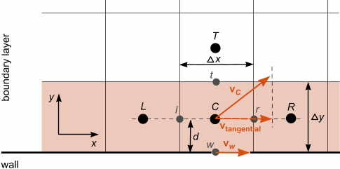
To derive the boundary conditions provided by the wall treatment in a simplified manner, consider the following 2D domain, where the wall is parallel to the $x$ -direction and the wall-normal direction is in the $y$ -direction:

For a steady-state flow with no external forces, the differential form of the transport equation for a scalar quantity $ϕ$ is given as:

Figure 1. EQUATION_DISPLAY

\frac{\partial}{\partial x} (ρ v ϕ) = \frac{\partial}{\partial y} (Γ \frac{\partial ϕ}{\partial y}) + S_{ϕ}

(1621)

where:

$ρ$ is the density.
$v$ is the velocity.
$Γ$ is the diffusion coefficient
$S_{ϕ}$ is the source term.

Integrating this equation over the volume of a near-wall cell gives the following equation:

Figure 2. EQUATION_DISPLAY

[{(ρ v ϕ)}_{r} - {(ρ v ϕ)}_{l}] Δy = [{(Γ \frac{\partial ϕ}{\partial y})}_{t} - {(Γ \frac{\partial ϕ}{\partial y})}_{w}] Δx + S_{ϕ} ΔxΔy

(1622)

where:

$r$ , $l$ , and $t$ indicate a value at the right, left, and top face of the near-wall cell, respectively. $w$ indicates a value at the wall.
$w$ indicates a value at the wall. $l$ , $t$ , and $r$ indicate a value at the left, top, and right face of the near-wall cell, respectively.
$Δx$ and $Δ y$ are the mesh size of the near-wall cell in x- and y-direction, respectively.

For momentum ( $ϕ = u, v$ ) and energy ( $ϕ = E$ ), the wall-normal gradient ${(Γ \frac{\partial ϕ}{\partial y})}_{w}$ corresponds to the wall shear stress $τ_{w}$ and the wall heat flux ${\dot{q}}_{w} ″$ , respectively.

Wall Shear Stress

For laminar flow, the wall-shear stress is calculated as:

Figure 3. EQUATION_DISPLAY

τ_{w} = μ {[{(\nabla v_{tangential})}_{C} + {(\nabla v_{tangential})}_{C}^{T}] - \frac{2}{3} {(\nabla\cdot v_{tangential})}_{C} I} n

(1623)

where:

Figure 4. EQUATION_DISPLAY

v_{tangential} = (v_{C} - v_{w}) - [(v_{C} - v_{w}) \cdot n] n

(1624)

and:

$C$ indicates a value at the centroid of the near-wall cell.
$μ$ is the dynamic viscosity.
$I$ is the identity tensor.
$n$ is the wall-normal unity vector.
$v_{w}$ is the velocity of the wall (zero for stationary walls).

The wall shear force is defined as:

Figure 5. EQUATION_DISPLAY

f_{w} = {- τ}_{w} A

(1625)

where $τ_{w}$ is the wall shear stress and $A$ is the boundary face area.

For turbulent flow, the wall shear stress must take into account the increase in shear stress due to turbulent mixing in the near-wall region. The applied method is based on the wall friction velocity $u_{τ}$ , from which the wall shear stress is computed as:

Figure 6. EQUATION_DISPLAY

τ_{w} = ρ u_{τ}^{2}

(1626)

The wall friction velocity $u_{τ}$ is calculated depending on the selected turbulence modeling approach, see Wall Treatment for Turbulence Models.

Wall Heat Flux

For laminar flow, the wall heat flux vector is calculated as:

Figure 7. EQUATION_DISPLAY

{\dot{q}}_{w} ″ = - k {(\nabla T)}_{C}

(1627)

where:

$k$ is the thermal conductivity of the fluid.
$T$ is the temperature.

The wall heat flux is then obtained from the wall heat flux vector as:

Figure 8. EQUATION_DISPLAY

{\dot{q}}_{w} ″ = | {\dot{q}}_{w} ″ |

(1628)

For turbulent flow, the wall heat flux is computed as:

Figure 9. EQUATION_DISPLAY

{\dot{q}}_{w} ″ = ρ C_{p} u_{*} \frac{{\hat{T}}_{C} - T_{w}}{{\hat{T}}_{C}^{+}}

(1629)

where $C_{p}$ is the specific heat.

The velocity scale $u_{*}$ and the non-dimensional RANS averaged/LES filtered cell temperature ${\hat{T}}_{C}^{+}$ are given by the wall treatment of the selected turbulence modeling approach. See Wall Treatment for Turbulence Models.