Home
Tutorials
Tutorials show you how to use Simcenter STAR-CCM+ for various applications in a step-by-step format with recommendations for setup, initialization and steps of the solution process specific to the application. Macro and simulation files are available for download for a large proportion of cases.
Incompressible Flow
The tutorials in this set illustrate various Simcenter STAR-CCM+ features for incompressible fluid flows as well as porosity and solution recording
Material Calibration: Curve Fitting Non-Newtonian Model Parameters
This tutorial illustrates the workflow for calibrating rheological model parameters from experimental rheological data through curve-fitting.
Generalized Newtonian Fluid: Power Law Model
In this section of the tutorial, set up the models and select the input data for the simulation of a generalized Newtonian fluid, then use the Fitting Tool from the Material Calibration model to obtain a fitted curve for shear rate versus shear viscosity. Use this curve to establish material properties.
Estimating Initial Values for the Power Law Parameters
Plot the imported experimental viscosity and examine the curve. This analysis allows you to provide good initial estimates for the curve-fitting algorithm, which are necessary to ensure convergence.

Share

Link: copied

Breadcrumb: copied

Tutorials
Tutorials show you how to use Simcenter STAR-CCM+ for various applications in a step-by-step format with recommendations for setup, initialization and steps of the solution process specific to the application. Macro and simulation files are available for download for a large proportion of cases.
- Using Tutorial Macros and Files
  Macros, input files, and final simulation files for a range of tutorials are provided as an optional download package on the Support Center website. These macros and final simulation files are provided as an aid to the written tutorials, so that you can check your final results against the downloaded files, or against a simulation that is built and run using the macros.
- Introduction
  Welcome to the Simcenter STAR-CCM+ introductory tutorial. In this tutorial, you explore the important concepts and workflow. Complete this tutorial before attempting any others.
- Foundation Tutorials
  The foundation tutorials showcase the major features of Simcenter STAR-CCM+ in a series of short tutorials.
- Geometry
  The tutorials in this set illustrate various Simcenter STAR-CCM+ features for creating and working with parts and 3D-CAD.
- Mesh
  The tutorials in this set illustrate various STAR-CCM+ features for building CFD meshes.
- Incompressible Flow
  The tutorials in this set illustrate various Simcenter STAR-CCM+ features for incompressible fluid flows as well as porosity and solution recording
  - Steady Flow: Lid-Driven Cavity Flow
    This tutorial demonstrates the performance of Simcenter STAR-CCM+ in solving a traditional square lid-driven cavity flow. The problem geometry consists of a two-dimensional 1 m² cavity. The cavity is covered by an impermeable wall that moves in the x-direction with constant velocity of 1 m/s. A stretched quadrilateral mesh with 6400 cells is used.
  - Steady Flow: Channel Flow with Multiple Meshes
    This tutorial describes a steady airflow simulation over an obstacle that is mounted at the bottom wall of a three-dimensional channel.
  - Steady Flow: Laminar and Turbulent Flow in an S-Bend
    This tutorial demonstrates the flow of an incompressible gas through an s-bend of constant diameter (2 cm), for both laminar and turbulent flow. The first part of the tutorial covers the laminar flow, with a Reynolds number (Re) of 500, and the second part covers the turbulent flow, Re = 50,000. The same pipe geometry is used in both cases.
  - Steady Flow: Backward Facing Step
    Steady flow over a backward facing step is a typical scenario to investigate the behaviour of reattaching flows. Understanding the behaviour of the flow is crucial for many applications such as designing heat exhangers, evalutating aerodynamic performance and improving flow control strategies.
  - Anisotropic Flow: Cyclone Separator
    The flow inside a cyclone separator is characterised by strong swirling motion and three-dimensional boundary layers. Properly accounting for these effects is a challenging problem for CFD simulations. This tutorial presents the initial step in setting up a coarse mesh cyclone flow simulation.
  - Porous Resistance: Isotropic Media
    This tutorial models flow through a catalyst geometry.
  - Porous Resistance: Orthotropic Media
    This tutorial solves the same problem as the Porous Resistance: Isotropic Media, except that the fluid in the porous region cannot flow in any direction other than the bulk flow (y-) direction.
  - Solution Recording and Playback: Vortex Shedding
    This tutorial demonstrates how to use the solution recording and playback module for capturing the results of transient phenomena.
  - Generalized Newtonian Fluid: Flow in a Static Mixer
    This tutorial demonstrates the process of setting up and analyzing the flow of a viscous fluid through a static mixer.
  - Viscoelastic Flow: Basic Extrusion
    This tutorial illustrates the extrusion of molten rubber through a die.
  - Material Calibration: Curve Fitting Non-Newtonian Model Parameters
    This tutorial illustrates the workflow for calibrating rheological model parameters from experimental rheological data through curve-fitting.
    - Prerequisites
      The Material Calibration: Curve Fitting tutorial assumes that you are already familiar with certain techniques in Simcenter STAR-CCM+.
    - Creating the Simulation and Importing the Experimental Data
      For this tutorial, you start from a new simulation. You import the tables containing the experimental data in .csv format. There is no need to include mesh or geometry.
    - Generalized Newtonian Fluid: Power Law Model
      In this section of the tutorial, set up the models and select the input data for the simulation of a generalized Newtonian fluid, then use the Fitting Tool from the Material Calibration model to obtain a fitted curve for shear rate versus shear viscosity. Use this curve to establish material properties.
      - Selecting the Physics Models and Materials
        Set up the physics continuum, then select physics models and data tables.
      - Defining the Rheological Data Type
        Define the rheological data type: specify that the imported table contains data of the type viscosity versus shear rate.
      - Estimating Initial Values for the Power Law Parameters
        Plot the imported experimental viscosity and examine the curve. This analysis allows you to provide good initial estimates for the curve-fitting algorithm, which are necessary to ensure convergence.
      - Curve-Fitting the Power Law Model
        Apply curve fitting to generate new parameter values and apply them to the simulaion.
    - Viscoelastic Fluid: Extended Pom-Pom Model
      In this section of the tutorial, modify the set of models and select the input data for the simulation of a viscoelastic fluid with the eXtended Pom-Pom (XPP) model, then use the Fitting Tool from the Material Calibration model to obtain a fitted curve.
    - Curing: Chemorheology Model
      In this section of the tutorial, you set up the models and select the input data for the simulation of a generalized Newtonian fluid that undergoes a curing process. You use the Chemorheology model to account for the changes in rheological properties due to that curing process.
  - Polymer Melt Extrusion: Film Casting
    In industry, film casting is a common process for producing thin polymeric films. Cast films are used for applications such as food and textile packaging, stretch wraps, or plastic bags. Simcenter STAR-CCM+ provides a combination of the Film Casting model and the Free Surface model that allows you to simulate that process and to investigate the impact of various parameters on the resulting film.
- Compressible Flow
  The tutorials in this set illustrate various Simcenter STAR-CCM+ features for compressible fluid flows as well as harmonic balance.
- Heat Transfer and Radiation
  The tutorials in this set illustrate various Simcenter STAR-CCM+ features for heat transfer, radiation, and thermal comfort.
- Multiphase Flow
  The tutorials in this set illustrate various Simcenter STAR-CCM+ features for simulating multiphase fluid flow problems
- Discrete Element Method
  The tutorials in this set illustrate various Simcenter STAR-CCM+ features for simulating Discrete Element Method problems
- Motion
  The tutorials in this set illustrate various STAR-CCM+ features for simulating problems with moving geometries and meshes, dynamic fluid body interaction, and rigid body motion:
- Reacting Flow
  The tutorials in this set illustrate various Simcenter STAR-CCM+ features for simulating reacting flows such as combustion.
- Solid Stress
  The tutorials in this set illustrate various Simcenter STAR-CCM+ features for computing deformation, strain, and stresses in solid regions. They also show how such computations can be coupled to the fluid behavior in an analysis of fluid-structure interaction.
- Aeroacoustics
  The tutorials in this set illustrate various Simcenter STAR-CCM+ features for solving aeroacoustic simulations.
- Electromagnetism
  The following tutorials illustrate features for solving problems that involve electromagnetic fields.
- Electrochemistry
  The following tutorial demonstrates chemical reactions induced by an electrical current.
- Battery
  The tutorials in this set illustrate various Simcenter STAR-CCM+ features for setting up a battery model:
- Automation
  The tutorials in this set illustrate various Simcenter STAR-CCM+ automation and macro features.
- Design Exploration
  The tutorials in this set illustrate various features for running design exploration studies in Design Manager.
- Coupling with CAE Codes
  The tutorials in this set illustrate various Simcenter STAR-CCM+ features for coupling with CAE codes:
- Analysis Methods
  The tutorials in this set illustrate various Simcenter STAR-CCM+ features for analysing and visualizing simulation data.
- Simcenter STAR-CCM+ In-cylinder
  The tutorials in this set illustrate features for simulating internal combustion engines in Simcenter STAR-CCM+ using the dedicated add-on Simcenter STAR-CCM+ In-cylinder.

Estimating Initial Values for the Power Law Parameters

Plot the imported experimental viscosity and examine the curve. This analysis allows you to provide good initial estimates for the curve-fitting algorithm, which are necessary to ensure convergence.

To estimate the initial values:

Right-click the Material Calibration node and select Fitting Tool....
The Material Parameter Fitting dialog opens.
Click on the Log Graph tab to display the log-log form of the graph.

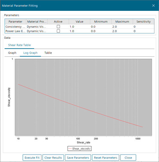
The displayed curve shows the imported shear viscosity as a function of shear-rate. It is recommended that you first deactivate all the model parameters and plot the data to see and analyze general behavior of the model. In this particular case, the experimental data shows shear thinning behavior, so the Power Law exponent should have a value between 0 and 1. Based on this observation, the initial value for the power law exponent is chosen to be 0.1 and the curve-fitting algorithm is bounded between 0 and 1. From the curve, the maximum shear viscosity is about 0.8. Therefore, an appropriate initial value for the consistency factor is 0.8. The consistency factor is bounded in a rational range between 0 and 3.

Enter the following settings in the parameters list.


Parameter	Value	Minimum	Maximum
Consistency Factor	0.8	0.0	3.0
Power Law Exponent	0.1	0.0	1.0

Click Execute Fit.
The curve displays the power law viscosity function using the initial values as model parameters. Curve-fitting only takes place when you activate Active.
Click Clear Results.