Elastoplastic Materials

For small strains, the strain tensor can be written as:

where ${\epsilon }_{el}$ is the elastic strain tensor, ${\epsilon }_{pl}$ is the plastic strain tensor, and ${\epsilon }_{in}$ includes any inelastic contribution to the strain tensor (for example, the thermal strain).

Following Eqn. (4503), the stress tensor can then be written as:

where $D$ is the material tangent. The energy that is dissipated due to plastic deformation can be written as:

where $\sigma$ is the Cauchy stress tensor.

A scalar measure of the plastic strain is the equivalent, or accumulated, plastic strain ${\epsilon }_{eq}$. This quantity represents the incremental plastic strain that is accumulated as the plastic damage increases:

Another scalar measure of plastic strain is the effective plastic strain ${\epsilon }_{eff}$, defined as:

To describe the stress-strain curve of elastoplastic materials, it is possible to define a function, called the plastic potential, such that:

The plastic potential is a function of the stress $\sigma$ and some hardening variables $\alpha$ (see Hardening Models). $f=0$ defines the yield surface:

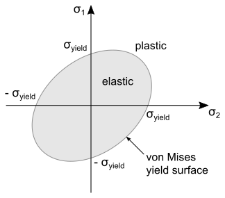
From Eqn. (4520), any stress state within the yield surface is elastic; any stress outside the yield surface is plastic. In general, the yield surface has the form:

where ${\sigma }^{*}$ is some measure of stress and ${\sigma }_Y$ is the material yield stress. For metals, the most common plastic potential is the J2 potential (also known as the von Mises potential), which is defined as:

Hardening Models

Hardening models describe how the yield surface changes with subsequent yielding. For example, for isotropic hardening, the yield surface remains centered about the same location, while expanding in size.

Simcenter STAR-CCM+ provides standard models for linear isotropic hardening and saturation hardening, as well as a user-defined hardening model.

Linear Isotropic Hardening

This model defines the yield stress ${\sigma }_Y$ as a linear function of the equivalent plastic strain ${\epsilon }_{eq}$:

$$\begin{array}{c}{\sigma }_Y\left({\epsilon }_{eq}\right)\end{array}={\sigma }_{Y_0}+H_0{\epsilon }_{eq}$$

(4523)

where ${\sigma }_{Y_0}$ is the initial yield stress and $H_0$ is the hardening tangent that defines the slope of the linear function.

For $H_0=0$, the yield stress is constant (${\sigma }_Y={\sigma }_{Y_0}$). This type of behavior is known as perfectly plastic.

Saturation Hardening

This model defines the yield stress ${\sigma }_Y$ as a nonlinear function of ${\epsilon }_{eq}$:

$$\begin{array}{c}{\sigma }_Y\left({\epsilon }_{eq}\right)\end{array}={\sigma }_{Y_0}+m\overline{H}{\epsilon }_{eq}+({\sigma }_{\infty }-{\sigma }_{Y_0})(1-e^{-\delta {\epsilon }_{eq}})$$

(4524)

where $m$ , $\overline{H}$ , ${\sigma }_{\infty }$ , and $\delta$ are parameters that can be found by curve-fitting material test data. The curve given by Eqn. (4524) approaches an asymptotic limit at higher strains:

User-Defined

This model allows you to capture the material behavior from experimental data. To define the stress-strain relationship, you specify the nominal stress $\sigma$ and its derivative with respect to the nominal strain $\epsilon$ :

$$\begin{array}{cc}\begin{array}{c}{\sigma }_Y\end{array};& \frac{\begin{array}{c}d{\sigma }_Y\end{array}}{d{\epsilon }_{eq}}\end{array}$$

(4525)

The nominal strain and nominal stress express the respective quantities in the undeformed configuration:

$$\sigma =\frac{F}{A_0}$$

(4526)

$$\epsilon =\frac{\delta L}{L_0}$$

(4527)

These nominal measures deviate from the true stress and strain values for large deformations, therefore, this model is suited to applications with small deformations.