Setting the Inlet and Outlet Boundary Conditions
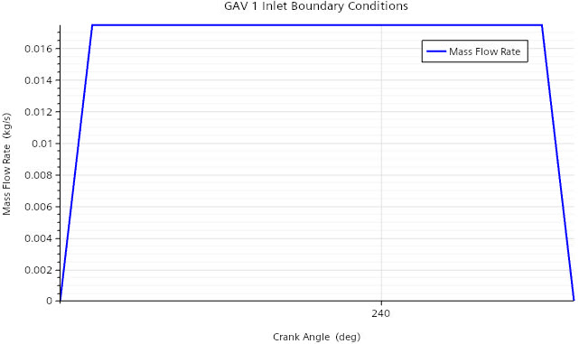
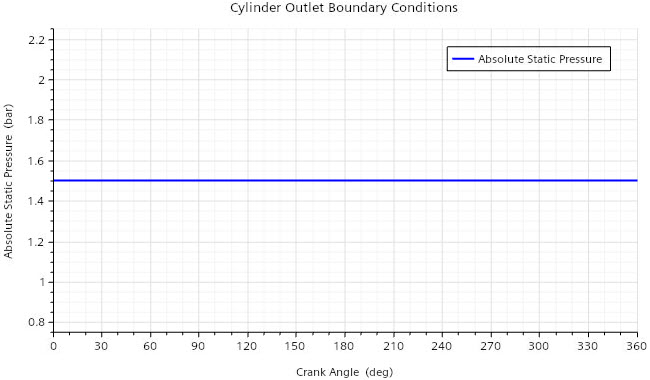
Air enters through the intake port inlet with a static temperature of 330 K and a pressure of 2.5 bar. At the inlets of the GAVs, you introduce methane gas with a total temperature of 330 K, where the gas admission starts at 230.0 deg CA and ends at 246.0 deg CA. You import a table that describes the mass flow rate of the methane gas as a function of crank angle. To avoid diffusion of flow quantities at the GAV inlets, you exclude the flow-boundary diffusion fluxes. At the exhaust port outlet, you set a pressure of 1.5 bar and a static temperature of 700 K.
-
Set the inlet boundary conditions for the intake port:
-
Set Temperature Column to T_K.
The plot in the Graphics window updates to add the temperature data—a constant temperature of 330 K for all crank angles.
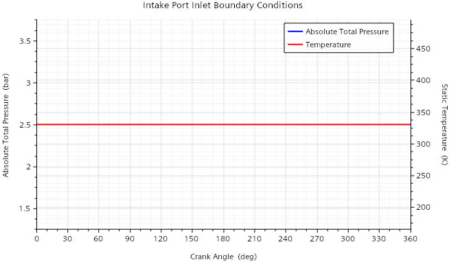
The correct species mass fractions for the inlet are set by default.
-
Set Temperature Column to T_K.
-
Set the inlet boundary conditions for the GAVs:
-
In the Import Table dialog,
navigate to the inCylinder folder of the downloaded tutorial
files, select twoStrokeEngine_GAV_Inlet.csv, and click
Open.
The correct table columns and units are assigned automatically.In the Graphics window, a plot opens that displays the mass flow rate as a function crank angle.
-
In the Import Table dialog,
navigate to the inCylinder folder of the downloaded tutorial
files, select twoStrokeEngine_GAV_Inlet.csv, and click
Open.
-
Exclude the flow-boundary diffusion fluxes:
-
Set the outlet boundary condition for the exhaust port:
-
In the Import Table dialog,
navigate to the inCylinder folder of the downloaded tutorial
files, select twoStrokeEngine_ExhaustPort_Outlet.csv, and click
Open.
In the Graphics window, a plot opens that displays a constant pressure of 1.5 bar for all crank angles.
-
In the Import Table dialog,
navigate to the inCylinder folder of the downloaded tutorial
files, select twoStrokeEngine_ExhaustPort_Outlet.csv, and click
Open.
-
Save the simulation
 .
.