Automobile Aerodynamics

At higher speeds, the aeroacoustic noise dominates noise from the engine, exhaust, and tires.

The aeroacoustic noise comes from air flows over pillars, wing-mirrors, and the underbody, and by flow through ducts (including fan noise). This section presents the following recommended practices to model automobile aerodynamics:

Recommended Process
Recommended Mesh Settings
Recommended Time-Step
Recommended Solver Settings

Recommended Process

Apply guidelines for mesh-resolution for a RANS-based steady state aerodynamics case. It is vital to get the mean flow correct. Compromise the wake refinement only if rear-vehicle aeroacoustics are not important.
Plot the mesh cut-off frequency to judge if the refinement in the acoustic source regions resolves frequencies in the region of 3–5 kHz. In practice, a mesh cell size of 2 mm or less is required. Refine appropriately and map the solution to the refined mesh.
You can identify the acoustic source regions from the regions where the acoustic correlations are large. Use Proudman for volume sources:

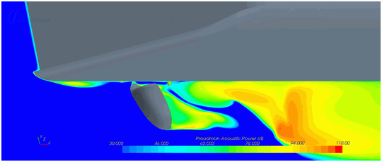
and Curle for surface sources: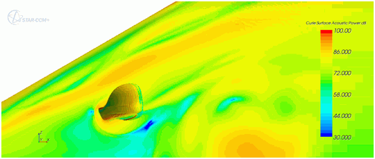
Ensure that the mesh in the near field is adequate for local sound propagation. For example, use 3.5 mm or less in the region of the A-pillar, side-view mirror, and side glass to propagate a 5 kHz signal.
Choose a time-step size suitable for the most demanding (that is, smallest) of the following constraints: frequency resolution, explicit CFL, or implicit CFL (as appropriate) and Courant number.
Restart a transient case from the initial steady state simulation that you used to judge the previous requirements. Switch the turbulence model from RANS to DES or LES. Use second-order time discretization, and a spatial discretization that is based on central differencing.
Select and fine-tune the numerical parameters to ensure convergence within each time-step. You can conclude that the solution has converged within a time-step when all (not a subset) of the following criteria are satisfied:
1. Monotonically reducing or minimized residuals at the end of the time-step.
2. An unchanging monitor. The monitor can be: pressure at a point, lift, or drag.

Recommended Mesh Settings

Select cell size,

Δ

, based on criteria:


Criterion	Comments / Description	Formula	Typical Values
Mean Flow	Use guidelines for external steady aerodynamics. Refine in the near-wall region to capture separation from the body.		$Δ_{\min}$ = 2 mm $y$ + = 1 for low-Re wall treatment
Turbulence integral scales, $L_{i n t e g r a l}$	A measure of the “typical” size of dissipative eddies. Approximated from steady state, $Δ \leq 0.5 L_{i n t e g r a l}$	$L_{i n t e g r a l} = \frac{C_{μ}^{0.75} \cdot k^{1.5}}{ϵ}$	$L_{i n t e g r a l}$ > 10 mm $Δ \leq 2$ mm
Frequencies that are associated with turbulent structures	Mesh cut-off frequency, that is based on local turbulent fluctuations compared to mesh size recommended in guidelines. Approximated from steady state.	$F_{M C F} = \frac{\sqrt{\frac{2}{3} k}}{2 Δ}$	$Δ$ = 4 mm captures frequencies in the range 1000–1500 Hz.
Propagation of pressure waves	Based on second order space and time discretization, 20 cells per acoustic wavelength, $λ$ (less for higher-order spatial schemes). $a$ , is the speed of sound.	$λ = \frac{a}{F}$ $Δ \leq \frac{λ}{20}$	$Δ \leq 3.5$ mm. Based on a requirement to propagate a pressure wave of $F$ = 5000 Hz in air.

Recommended Time-Step

Select the time-step size

Δ t

, based on criteria:


Criterion	Comments / Description	Formula	Typical Values
A signal of frequency $F$	The Nyquist sampling theorem states that a signal with frequency, $F$ , can be resolved by sampling at a rate greater than $2 F$ . For second-order spatial schemes, tests show that around 15 points are required to resolve the wave amplitude.	$Δ t_{F} \leq \frac{1}{15 F}$ , recommended	$Δ t_{F}$ = 2.22E-5 s. Based on requirement to capture $F$ = 3000 Hz.
Convection and acoustics	Based on the convection speed, $U$ , and speed of sound (acoustic pressure waves propagate at the local speed of sound, $a$ ). The Courant (CFL) number is based on $(U + a)$	Explicit: $Δ t_{e x p} = \frac{Δ}{(U + a)}$ Implicit: $Δ t_{i m p} = C F L \cdot Δ t_{e x p}$	$Δ t_{e x p}$ = 5.0E-6 s. Based on $Δ$ = 2.0 mm, $U$ = 50 m/s and $a$ = 350 m/s. $Δ t_{i m p}$ = 5.0E-5 s. Based on $C F L$ = 10.
Convection only	Based on convection speed, $U$ . Convective Courant Number is based on $U$ only.	${Δ t}_{C o u r a n t} = \frac{Δ}{U}$	$Δ t_{C o u r a n t}$ = 4.0E-5 s. Based on $Δ$ = 2.0 mm and $U$ = 50 m/s.
Diffusive time-scales	Most important in the boundary layer where the local (eddy) viscosity, $V_{e f f}$ , is largest. Unimportant to acoustic phenomena	${Δ t}_{d i f f} = \frac{Δ_{n o r m a l}^{2}}{V_{e f f}}$	$Δ t_{d i f f}$ = 1.0E-6 s. Based on $Δ_{n o r m a l}$ = 5.0E-6 m, $V_{e f f}$ = 2.0E-5 m²/s.

Recommended Solver Settings

You can select solver settings for a slower (“regular”) mesh and time-step setup, a faster (“aggressive”) setup, or the default settings.


	Velocity URF	Pressure URF	# Iterations Per Time step
Default	0.8	0.2	5
Regular $Δ t$ = 1.0E-4 to 1.0E-5 s. $Δ_{m i n}$ = 1–4 mm.	0.7	0.7	4–10
Aggressive $Δ t$ = 2.0E-5 s. $Δ_{m i n}$ = 2 mm.	1.0	0.9	3