Design Manager provides three data sets by which
you can assess the accuracy of the surrogate prediction.
To assess how well the computed
surrogate function fits the known sample data, for each design response, you compare the
actual values from the simulations with the predicated values from surrogate. You can
visualize the comparison through a surrogate fit plot. A high accuracy is
assessed when the predicted values are very close to the simulated values. To assess how well the surrogate
function fits the unknown data, you do a cross validation for the surrogate to
evaluate its prediction reliability for the entire design space. For each response,
you evaluate the cross validation residuals in the residual table. You can also
create an Actual vs Residual Plot to visualize the residuals. Due to the
randomness of the cross validation scheme, you are advised to perform cross
validation multiple times.
The
predicted residual error sum of squares (PRESS) residuals are another means by which
to assess the accuracy of the surrogate model predictions. The PRESS residual is
equivalent to the Leave-one-out cross validation, and it is also equivalent to the
K-Fold cross validation scheme when the Cross
Validation K-Fold Value is set to
1. For PRESS you only perform one cross validation as
there are no random groupings and the PRESS residuals remain fixed. Generally, you
are advised to look at both types of residuals as each of them has its predictive
power. See also: Cross Validation Scheme.
For the surrogate types
Kriging and RBF, the cross
validation and PRESS residuals are the values to judge the accuracy of the surrogate
prediction. Since the structure of the surrogate function defines the exact fit of
the known data, correlation coefficient (R2) and adjusted correlation coefficient
(R2adj) are naturally equal to 1. See also: Kriging,
Radial Basis Function and Cross Validation.
-
To create surrogate fit plots:
-
Right-click on the and select .
-
In the Surrogate Fit Plot Setup dialog, select the
surrogate for which you want to create a surrogate fit plot.
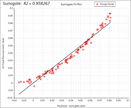
An example of
surrogate fit plot of a Least Squares surrogate type is shown
below:
The reference line
y=x gives an indication of how close
predicted response values from the bottom axis match the actual
response values from the left vertical axis.
If you are not
satisfied with the match of predicted to actual response values, you
can try modifying surrogate settings and recomputing the surrogate
without re-running the design study.
-
To run a cross validation and assess the accuracy of surrogate residuals:
-
Select the node and specify the three following properties:
- Cross Validation
Scheme
- Cross Validation
K-Fold Value
- Cross Validation
Seed
For more details
regarding property settings, refer to Cross Validation Scheme.
-
Right-click the [surrogate] node and select
Cross
Validate.
-
Right-click the [surrogate] node and select
Open Residual
Table.
A residual table of a surrogate is shown below. The
marked column displays the cross validation residuals, which indicate
how precise the surrogate predicts new, unknown response values.
-
To visualize the cross validation residual, right-click the node and select .
-
In the Actual vs Residual Plot Setup dialog,
select the surrogate for which you want to create a surrogate fit
plot.
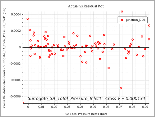
Beside the small
residual value, tightly scattered residuals around the zero
reference line indicate also a good prediction accuracy of this
surrogate.
The marked annotation
is the root mean square (RMS) of all cross validation residuals in
the Cross V Residual column—the lower the
value, the better the fit.
-
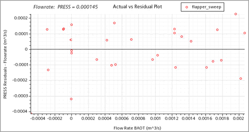
To visualize the PRESS values—the Predicted Error Sum of Squared
values, right-click the node and select .
-
Select the node and set Values
Type to PRESS
Residuals.
The Cross V and PRESS
residuals are an estimate error you expect in predicted values. The
fact that the relative errors of both residuals are small and
consistent over several cross validations indicates that the
surrogate model has a good prediction accuracy over the design
space.
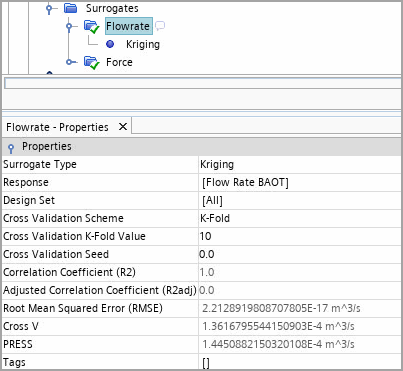
Beside the Cross V and PRESS residuals, you also evaluate the
Correlation Coefficient
(R2) and Root Mean Squared
Error (RMSE) of the surrogate. If R2 is not 1 or RMSE is not near zero, then the surrogate model is seen
as numerically ill-conditioned. It leads to a loss of precision and a poor fit to
the data.
-
To check the R2 and
RMSE values, select the and check the read-only values.


