Curve-Fitting the Linear Model Parameters for One Mode
To calibrate the model parameters for viscoelastic models, start with the linear parameters polymer relaxation time and polymer viscosity. As before, deactivate all the model parameters, then plot and analyze the general fluid behavior.
Use the logarithmic plot of the experimental , curves to obtain estimate initial values for the linear model parameters: the polymer viscosity and the relaxation time. In the plot, you find the intersection point of the two curves. Then, you read off the values for and the frequency from the x and y axes. By applying the following rules of thumb, you obtain suitable initial values for the curve-fitting algorithm:
Initial relaxation time:
Initial polymer viscosity:
For the minimum and maximum values of relaxation time and viscosity , use a rational range, generally starting from one decade smaller for minimum to one decade larger for the maximum.
More exact values for the minimum and maximum values of the polymer relaxation time and viscosity can be calculated using following relationships:
- where is the highest frequency on the frequency vs GpGpp curves.
- where is the lowest frequency on the frequency vs GpGpp curves.
- where and are the frequencies for the respective and values.
- .
To curve-fit the linear model parameters:
-
Under Extended Pom-Pom, right-click on the
Material Calibration node and select
Fitting Tool....
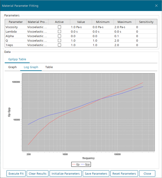
The Material Parameter Fitting dialog displays. The graph shows the imported curves of storage modulus and loss modulus.
-
Select the Log Graph tab to display the
log-log version of the graph.
-
Examine the displayed curve. Note that the Gp and
Gpp curves intersect at a frequency of 4000/s,
where Gp= Gpp= 32,000
Pa.
The initial value for Lambda is 1/4000 s = 0.00025 s.
The initial value for Viscosity is 2 · 32,000 Pa · 0.00025 s = 16 Pas.
-
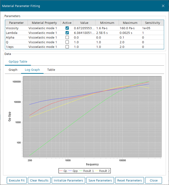
Enter the initial values, minima, and maxima for Viscosity and Lambda as given below.
It is good practice to specify the minima and maxima as a decade below and above the initial values.
Parameter Value Minimum Maximum Viscosity 16 Pa-s 1.6 Pa-s 160 Pa-s Lambda 0.00025 s 0.000025 s 0.0025 s -
Activate the Viscosity and
Lambda parameters by
selecting Active and click Execute
Fit.
The curve-fitting algorithm is invoked.Note that the Result 1 and Result 2 curves do not coincide with the Gp and Gpp curves, based on the optimization engine for the single mode viscoelastic model they are the best candidates in frequency spectrum.
- Click Clear Results and Reset Parameters to restore the initial state of the curve fitting.
- Deactivate the Viscosity and Lambda parameters
- Click Close to close the dialog.
- Save the simulation.
The following sections add two more modes to extend the search for a better fit.