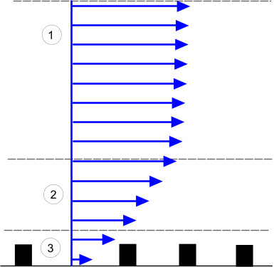
Atmospheric Boundary Layers

The Atmospheric Boundary Layer (ABL) is an important part of simulating wind and is used in modeling weather and wind-borne pollution, and in designing wind-farms.

The ABL is the bottom layer of the atmosphere, in contact with the surface of the Earth. Within this layer, features of the surface of the Earth directly affects flow: frictional effects and temperature create turbulence and vertical mixing. Above this layer, rotational effects, rather than turbulence, dominate the flow. The depth of the ABL can vary in both time and space.

Garratt [347] decomposes the boundary layer in the atmosphere of the Earth into two sublayers:

An outer Ekman sublayer where there is little dependence on the nature of the surface.
An inner sublayer where surface effects such as friction and heating are important.

There is an interfacial sublayer within this inner layer that defines the height and the structure (together termed roughness) of obstacles to the flow on the ground.


Index	Description
1	Ekman sublayer
2 & 3	Inner sublayer
3	Interfacial sublayer

In the literature, the preferred method of modeling the roughness of an atmospheric boundary layer is to use the Richard and Hoxey Law [349]. This method is based on the following premises:

Vertical velocity is zero.
Pressure is constant.
Shear stress is constant.
The K-Epsilon turbulence model is in equilibrium.

Atmospheric boundary layers can be modeled in conjunction with any turbulence model. However, for the Standard K-Epsilon turbulence model, the Atmospheric Boundary Layer model allows you to set inlet boundary profiles according to the Richard and Hoxey Law.

The K-Epsilon turbulence model in equilibrium gives the following solutions for the stream-wise velocity component $u$ , turbulent kinetic energy $k$ and turbulent dissipation rate $ϵ$ , valid throughout the domain:

Figure 1. EQUATION_DISPLAY

u = \frac{u_{*}}{κ} \ln (\frac{y_{0} + y}{y_{0}})

(1372)

Figure 2. EQUATION_DISPLAY

k = \frac{u_{*}^{2}}{\sqrt{C_{μ}}}

(1373)

Figure 3. EQUATION_DISPLAY

ε = \frac{u_{*}^{3}}{κ (y + y_{0})}

(1374)

where:

$κ$ is von Karman's constant, recommended value 0.42.
$y_{0}$ is the surface roughness length.
$y$ is the wall distance to the nearest wall.
$C_{μ}$ is a parameter of the K-Epsilon turbulence model, recommended value 0.013.

$u_{*}$ is the friction velocity:

Figure 4. EQUATION_DISPLAY

u_{*} = \frac{κ u_{h}}{\ln (\frac{h + y_{0}}{y_{0}})}

(1375)

where $u_{h}$ is a specified velocity at a reference height $h$ .

For ABL simulations, the flows are predominantly turbulent, and the velocity distribution maps to Eqn. (1603) in Simcenter STAR-CCM+. Following Martinez [348], let Eqn. (1375) equal Eqn. (1603), and cancel the common terms to give:

Figure 5. EQUATION_DISPLAY

\frac{y_{0} + y}{y_{0}} = E^{'} y^{+}

(1376)

Substitute $E^{'}$ using Eqn. (1604) and Eqn. (1640) for rough walls ( $R^{+} > 90$ , $B = 0$ ):

Figure 6. EQUATION_DISPLAY

\frac{y_{0} + y}{y_{0}} = \frac{{E y}^{+}}{C R^{+}}

(1377)

Substitute $y^{+}$ using Eqn. (1584) and $R^{+}$ using Eqn. (1639). Cancel common terms, giving:

Figure 7. EQUATION_DISPLAY

\frac{y_{0} + y}{y_{0}} = \frac{E y}{C r}

(1378)

Finally, assume that $y ≫ y_{0}$ , so that:

Figure 8. EQUATION_DISPLAY

\frac{y}{y_{0}} = \frac{E y}{C r}

(1379)

Canceling common terms provides the relation to modify the Simcenter STAR-CCM+ wall roughness equations to model an ABL:

Figure 9. EQUATION_DISPLAY

r = \frac{E y_{0}}{C}

(1380)

where:

$E$ and $C$ are wall function coefficients.

To guarantee physical results, ( $u^{+} > 0$ ) make sure that $y ≫ y_{0}$ is satisfied, in particular at wall cells (i.e. wall distances to wall-cell centroids are larger than the roughness length), and deactivate the Roughness Limiter wall roughness parameter.