Body Connections

Spring-Damper Coupling

The spring damper coupling connects two bodies, or one body and the environment, with an elastic force and a damping force, where the elastic part is given by Hooke's law. The total force on the end points is:

Figure 1. EQUATION_DISPLAY

\begin{array}{l} f_{1} (x) = k_{e f f} (x - x_{0}) + k_{d} \dot{x} \\ f_{2} (x) = - f_{1} (x) \end{array}

(4944)

Here, $f_{1}$ is the force acting at the first end point position vector $x_{1}$ . $f_{2}$ is the reaction force acting at the second end point position vector $x_{2}$ . $x$ is the distance (scalar) between the two end points. $x_{0}$ is the distance where the elastic force vanishes (relaxation length of the spring). $k_{e f f}$ is the effective elastic coefficient, and $k_{d}$ is the damping coefficient. The rate of change of the distance $\dot{x}$ is the relative velocity of the two end points. It is positive if the end points move apart, and negative if they approach.

The direction of the forces is given by the normalized direction vector $d$ from the first to the second end point:

Figure 2. EQUATION_DISPLAY

\begin{array}{l} d = (x_{2} - x_{1}) / | x_{2} - x_{1} | \\ f_{1} = f_{1} \cdot d \\ f_{2} = f_{2} \cdot d \end{array}

(4945)

In these equations, $x_{1}$ is the location to which the first end of the spring is attached and $x_{2}$ is the opposite end of the spring.

The elastic force $f_{e}$ is defined using the effective elastic coefficient $k_{e f f}$ :

Figure 3. EQUATION_DISPLAY

f_{e} (x) = k_{e f f} (x) \cdot (x - x_{0})

(4946)

Here, $f_{e}$ is the elastic force on the first end point.

The most simple case is a linear elastic force law— $f_{e} (x) = k \cdot (x - x_{0})$ with a constant effective elastic coefficient $k$ .

For the general case of a non-linear elastic force law, the effective coefficient can be computed based on the known $f_{e} (x)$ :

Figure 4. EQUATION_DISPLAY

k_{e f f} (x) = \frac{f_{e} (x)}{x - x_{0}}, x \neq x_{0}

(4947)

For $x = x_{0}$ , you can use $k_{e f f} (x_{0}) = k (x_{0})$ , where $k (x) = \frac{ⅆ f_{e} (x)}{ⅆ x}$ is the non-linear stiffness of the spring.

If the spring stiffness $k (x)$ is known, the following equation can be used to compute $k_{e f f}$ :

Figure 5. EQUATION_DISPLAY

k_{e f f} (x) = \frac{\int_{x_{0}}^{x} k (x´) ⅆ x´}{x - x_{0}}, x \neq x_{0}

(4948)

Similar as the equation above, for $x = x_{0}$ , you can use $k_{e f f} (x_{0}) = k (x_{0})$ .

In some applications, the relaxation length $x_{0}$ is outside of the operational range of the spring, and it may even be unknown. In such cases, an arbitrary value $x_{0}$ outside of the spring's operational range can be chosen, and the effective coefficient can be computed as:

Figure 6. EQUATION_DISPLAY

k_{e f f} (x) = \frac{{f_{r} + \int}_{x_{r}}^{x} k (x´) ⅆ x´}{x - x_{0}}, x \neq x_{0}

(4949)

Here, $f_{r}$ is some reference force on the first end point at the reference distance $x_{r}$ . Distances from $x_{r}$ to $x$ must be in the spring's operational range, while $x_{0}$ is somewhere outside.

An example for a non-linear spring with relaxation length $x_{0}$ and effective elastic coefficient $k_{e f f} (x)$ is:

Figure 7. EQUATION_DISPLAY

k_{e f f} (x) = a + b (x - x_{0}) + c {(x - x_{0})}^{2}

(4950)

Here, $a$ , $b$ and $c$ are constant values. The elastic force on the first end point of the spring is:

Figure 8. EQUATION_DISPLAY

f (x) = k_{e f f} (x) \cdot (x - x_{0}) = a (x - x_{0}) + b {(x - x_{0})}^{2} + c {(x - x_{0})}^{3}

(4951)

The terms for $k_{e f f} (x)$ and $f (x)$ are polynomials in $(x - x_{0})$ .

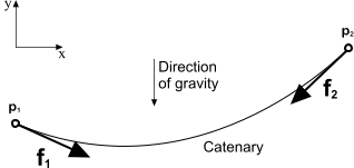
Catenary Coupling

The catenary coupling models an elastic, quasi-stationary catenary (such as a chain or towing rope), which is hanging between two end points, being subject to its own weight in the gravity field. In a local Cartesian coordinate system, the shape of the catenary is given by the following set of parametric equations:

Figure 9. EQUATION_DISPLAY

\begin{matrix} x = a u + b \sinh (u) + α \\ y = a \cosh (u) + \frac{b}{2} \sinh^{2} (u) + β \\ for u_{1} \leq u \leq u_{2} \end{matrix}

(4952)

where:

$a = \frac{c}{λ_{0} g}$

$b = \frac{c a}{D L_{e q}}$

$c = \frac{λ_{0} L_{e q} g}{\sinh (u_{2}) - \sinh (u_{1})}$

In these equations, $g$ is the gravitational acceleration, $λ_{0}$ and $L_{e q}$ are the mass per unit length and the relaxation length of the catenary, respectively, under force-free conditions. $D$ is the stiffness of the catenary, and $α$ and $β$ are integration constants depending on the position of the two end points and the total mass of the catenary. The curve parameter $u$ is related to the inclination angle $ϕ$ of the catenary curve by the following equation:

Figure 10. EQUATION_DISPLAY

\tan ϕ = \sinh (u)

(4953)

The parameter values $u_{1}$ and $u_{2}$ represent the positions of the catenary’s end points $p_{1}$ and $p_{2}$ in parameter space.

The forces $f_{1}$ and $f_{2}$ acting at the two end points of the catenary are directed along the local tangent vectors of the catenary curve at the parameter values $u_{1}$ and $u_{2}$ , respectively. They are given by the following expressions:

Figure 11. EQUATION_DISPLAY

\begin{array}{l} f_{1, x} = c \\ f_{1, y} = c \sinh (u_{1}) \end{array}

(4954)

and

Figure 12. EQUATION_DISPLAY

\begin{array}{l} f_{2, x} = - c \\ f_{2, y} = - c \sinh (u_{2}) \end{array}

(4955)

These forces, and the resulting catenary curve, are illustrated in the diagram below.

Contact Coupling

For continuum bodies, the contact coupling prevents contact of the boundary associated with the rigid body with another boundary, which can be either a boundary of the computational domain (body-environment coupling) or the boundary associated with another continuum body (body-body coupling).

To prevent contact, the model applies a contact force that depends on the distance between the rigid body boundary and the opposing boundary. The contact force decreases to zero when the distance between the body boundary and the other boundary is larger than a user-specified effective range. If the distance is smaller than the effective range, a repulsive contact force is applied.

The contact force on boundary face $f$ can be written as:

Figure 13. EQUATION_DISPLAY

f_{f} = f_{n} + f_{t}

(4956)

where $f_{n}$ is the normal component, which prevents contact, and $f_{t}$ is the tangential component, which models the friction of the body sliding along the opposing boundary.

The contact force results in a moment $m_{f}$ around the current body position $r_{b}$ :

Figure 14. EQUATION_DISPLAY

m_{f} = (r_{f} - r_{b}) \times f_{f}

(4957)

where $r_{f}$ is the location of the face centroid of face $f$ . The total force and the total moment on the body are each the sum of all contributions of all faces of the body surface.

The normal component of the contact force can be written as:

Figure 15. EQUATION_DISPLAY

f_{n} (d_{f}) = a_{f} [k_{1} (d_{0} - d_{f}) - k_{2} {\dot{d}}_{f}] n_{b f}

(4958)

where $k_{1}$ is the elastic coefficient, $k_{2}$ is the damping coefficient, $a_{f}$ is the face area, $d_{f}$ is the distance between the face centroid and the opposing boundary, $d_{0}$ is the effective range, and $n_{b f}$ is the normal of the boundary face next to face $f$ .

The elastic coefficient

k_{1}

is essential to stop the rigid body before contact is made. To estimate a value for this coefficient in case of impact, the following relations apply:

Body-body couplings:
Figure 16. EQUATION_DISPLAY

$k_{1} = \frac{m_{1} m_{2}}{m_{1} + m_{2}} \cdot \frac{1}{A} \cdot \frac{v_{n, r e l}^{2}}{{(d_{0} - d_{m i n})}^{2}}$
(4959)
Body-environment couplings:

Figure 17. EQUATION_DISPLAY

k_{1} = \frac{m_{1}}{A} \cdot \frac{v_{n, r e l}^{2}}{{(d_{0} - d_{m i n})}^{2}}

(4960)

where $m_{1}, m_{2}$ denote the masses of body 1 and 2, $A$ is the estimated area of contact, $v_{n, r e l}$ is the normal relative impact velocity of the two coupled objects, and $d_{m i n}$ is the minimum distance. The body should stop before this distance is reached.

The time required for stopping the body by applying the contact force is estimated as follows:

Body-body couplings:
Figure 18. EQUATION_DISPLAY

$τ = \frac{π}{2} \sqrt{\frac{m_{1} \cdot m_{2}}{(m_{1} + m_{2}) A k_{1}}}$
(4961)
Body-environment couplings:
Figure 19. EQUATION_DISPLAY

$τ = \frac{π}{2} \sqrt{\frac{m_{1}}{A k_{1}}}$

(4962)

To resolve the stopping process, the simulation time-step must be sufficiently smaller than $τ$ . Alternatively, the 6-DOF Solver can use sub-stepping. The above relations are only valid for weak damping.

To estimate a value for the damping coefficient, the following relations apply:

Body-body coupling:
Figure 20. EQUATION_DISPLAY

$k_{2} = 2 ς \sqrt{\frac{{(m}_{1} \cdot m_{2}) k_{1}}{(m_{1} + m_{2}) A}}$

(4963)
Body-environment coupling:
Figure 21. EQUATION_DISPLAY

$k_{2} = 2 ς \sqrt{\frac{m_{1} k_{1}}{A}}$
(4964)

where $ς$ is a constant factor describing the amount of damping. In general, $ς$ should be sufficiently small ( $ς ≪ 1$ ), as large values of $ς$ in combination with a large time-step can cause numerical instability.

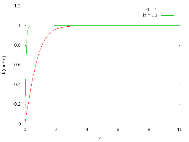
The tangential component of the contact force on face $f$ is given by:

Figure 22. EQUATION_DISPLAY

f_{t} = - μ | f_{n} | \tanh (k_{t} v_{t})

(4965)

where $μ$ is the friction coefficient, $k_{t}$ is the tanh coefficient, and $v_{t}$ is the tangential velocity of face $f$ relative to the opposing boundary.

This tangential force component models the kinetic friction between the body and the boundary. Static friction is not accounted for. The tanh function makes the friction force stable for small relative sliding velocities.

For sliding velocities $v_{t} ≫ 1 / k_{t}$ , the friction force depends only on the friction coefficient, the normal force, and the direction of the relative velocity. Depending on $k_{t}$ , the friction force remains constant with increasing sliding velocity. For smaller sliding velocities, the friction force additionally depends on the velocity magnitude.