Home
Tutorials
Tutorials show you how to use Simcenter STAR-CCM+ for various applications in a step-by-step format with recommendations for setup, initialization and steps of the solution process specific to the application. Macro and simulation files are available for download for a large proportion of cases.
Aeroacoustics
The tutorials in this set illustrate various Simcenter STAR-CCM+ features for solving aeroacoustic simulations.
DES and FW-H On-The-Fly: Noise from a Cylinder (Unsteady Analysis)
In the previous section of this tutorial, you completed the steady-state analysis runs for qualifying the volume mesh. In this section, continuing from the previous simulation file, you set up the final transient run for an unsteady analysis of the near field and an FW-H analysis of the far field.
Performing the Spectral Analysis
Using Fast Fourier Transforms, you can determine sound pressure as a function of frequency at each of the point receivers.

Share

Link: copied

Breadcrumb: copied

Tutorials
Tutorials show you how to use Simcenter STAR-CCM+ for various applications in a step-by-step format with recommendations for setup, initialization and steps of the solution process specific to the application. Macro and simulation files are available for download for a large proportion of cases.
- Using Tutorial Macros and Files
  Macros, input files, and final simulation files for a range of tutorials are provided as an optional download package on the Support Center website. These macros and final simulation files are provided as an aid to the written tutorials, so that you can check your final results against the downloaded files, or against a simulation that is built and run using the macros.
- Introduction
  Welcome to the Simcenter STAR-CCM+ introductory tutorial. In this tutorial, you explore the important concepts and workflow. Complete this tutorial before attempting any others.
- Foundation Tutorials
  The foundation tutorials showcase the major features of Simcenter STAR-CCM+ in a series of short tutorials.
- Geometry
  The tutorials in this set illustrate various Simcenter STAR-CCM+ features for creating and working with parts and 3D-CAD.
- Mesh
  The tutorials in this set illustrate various STAR-CCM+ features for building CFD meshes.
- Incompressible Flow
  The tutorials in this set illustrate various Simcenter STAR-CCM+ features for incompressible fluid flows as well as porosity and solution recording
- Compressible Flow
  The tutorials in this set illustrate various Simcenter STAR-CCM+ features for compressible fluid flows as well as harmonic balance.
- Heat Transfer and Radiation
  The tutorials in this set illustrate various Simcenter STAR-CCM+ features for heat transfer, radiation, and thermal comfort.
- Multiphase Flow
  The tutorials in this set illustrate various Simcenter STAR-CCM+ features for simulating multiphase fluid flow problems
- Discrete Element Method
  The tutorials in this set illustrate various Simcenter STAR-CCM+ features for simulating Discrete Element Method problems
- Motion
  The tutorials in this set illustrate various STAR-CCM+ features for simulating problems with moving geometries and meshes, dynamic fluid body interaction, and rigid body motion:
- Reacting Flow
  The tutorials in this set illustrate various Simcenter STAR-CCM+ features for simulating reacting flows such as combustion.
- Solid Stress
  The tutorials in this set illustrate various Simcenter STAR-CCM+ features for computing deformation, strain, and stresses in solid regions. They also show how such computations can be coupled to the fluid behavior in an analysis of fluid-structure interaction.
- Aeroacoustics
  The tutorials in this set illustrate various Simcenter STAR-CCM+ features for solving aeroacoustic simulations.
  - Broadband Models: Noise from a Cylinder (Preparation)
    This tutorial demonstrates how to set up aeroacoustics problems in Simcenter STAR-CCM+. The flow around a cylinder is used in the simulation to describe the required steps.
  - DES and FW-H On-The-Fly: Noise from a Cylinder (Unsteady Analysis)
    In the previous section of this tutorial, you completed the steady-state analysis runs for qualifying the volume mesh. In this section, continuing from the previous simulation file, you set up the final transient run for an unsteady analysis of the near field and an FW-H analysis of the far field.
    - Loading the Initial Simulation
      The steady-state analysis runs are now complete. Set up the final transient run.
    - Selecting the Transient Calculation Physics Models
      Modify the physics model selections to activate the unsteady solver.
    - Setting the Solver Properties and Stopping Criteria
      Choosing the correct time-step is an important step in setting up an aeroacoustic simulation.
    - Visualizing the Mean Velocity
      Create a monitor for displaying the mean velocity magnitude in a scalar scene.
    - Monitoring Pressure
      Create three probes that are used to monitor pressure while the solvers are running.
    - Monitoring Force Coefficients
      By default Simcenter STAR-CCM+ provides a residuals plot which can be used to monitor the convergence of the solution.
    - Setting Up the Solution History File
      To save solution data at regular intervals while the simulation is running, you create a solution history file (.simh). In this tutorial, you save the pressure data on the cylinder wall and on the plane section, so that you can perform surface spectral analysis after the simulation completes.
    - Preparing the On-The-Fly FW-H Analysis
      The two key steps in preparing Simcenter STAR-CCM+ for a Ffowcs Williams-Hawkings analysis are to define the FW-H Surfaces and then define the FW-H Receivers. FW-H Receivers are points at specific distances from the noise sources.
    - Visualizing the Solution
      Add scenes for the noise emitted from the cylinder surface and received at each receiver.
    - Running the Simulation
      The simulation is now ready to be run. It is best that you run this simulation in parallel using several CPUs, as otherwise the run time is considerable.
    - Visualizing the Results
      You can now visualize the acoustic pressure on the cylinder, based on input from the two point-receivers.
    - Performing the Spectral Analysis
      Using Fast Fourier Transforms, you can determine sound pressure as a function of frequency at each of the point receivers.
    - Results Analysis
      Compare the peaks in the spectra with the Mesh Frequency Cutoff plot from the final steady-state simulation.
    - Summary
      This tutorial continued from the previous one, doing an unsteady analysis of the near field and an FW-H analysis of the far field.
    - DES and FW-H On-The-Fly Tutorial Bibliography
  - Ffowcs Williams-Hawkings: Sound Propagation
    This tutorial compares the Post FW-H model with the FW-H On-The-Fly model.
  - Signal Post-Processing: FFT and Wavenumber
    Several further analyses are possible using the simulation history file from the earlier tutorial, DES and FW-H On-The-Fly: Noise from a Cylinder (Unsteady Analysis). These analyses are covered in this tutorial.
  - Acoustic Wave Modeling: Noise from a Cylinder
    This tutorial demonstrates how to set up an acoustic wave simulation in Simcenter STAR-CCM+. The flow around a cylinder is used in the simulation to describe the required steps.
  - Lighthill Wave and Perturbed Convective Wave Modeling: Simplified HVAC Duct
    Noise generated by the air handling components in heating, ventilation, and air conditioning (HVAC) systems is a large contributor to interior cabin sound levels. Investigating the sources of noise and modifying the design accordingly, leads to better and quieter systems.
  - Sponge Layer Modeling: Simplified Tailpipe
    Unsteady aeroacoustics simulations require effective non-reflective boundary conditions to prevent spurious reflected acoustic waves from the boundaries of the computational domain interfering with the aeroacoustic results.
- Electromagnetism
  The following tutorials illustrate features for solving problems that involve electromagnetic fields.
- Electrochemistry
  The following tutorial demonstrates chemical reactions induced by an electrical current.
- Battery
  The tutorials in this set illustrate various Simcenter STAR-CCM+ features for setting up a battery model:
- Automation
  The tutorials in this set illustrate various Simcenter STAR-CCM+ automation and macro features.
- Design Exploration
  The tutorials in this set illustrate various features for running design exploration studies in Design Manager.
- Coupling with CAE Codes
  The tutorials in this set illustrate various Simcenter STAR-CCM+ features for coupling with CAE codes:
- Analysis Methods
  The tutorials in this set illustrate various Simcenter STAR-CCM+ features for analysing and visualizing simulation data.
- Simcenter STAR-CCM+ In-cylinder
  The tutorials in this set illustrate features for simulating internal combustion engines in Simcenter STAR-CCM+ using the dedicated add-on Simcenter STAR-CCM+ In-cylinder.

Performing the Spectral Analysis

Using Fast Fourier Transforms, you can determine sound pressure as a function of frequency at each of the point receivers.

To perform the spectral analysis.

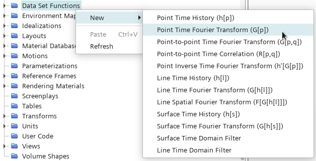
Right-click the Tools > Data Set Functions node and select New > Point Time Fourier Transform (G(p)).

Select the G(p) 1 node and set the following properties:


Property	Value
Start Time	0.02 s
Cut-off Time	0.0533 s
Amplitude Function	Sound Pressure Level
Analysis Blocks	2
Overlap Factor	0.5
Window Function	Hann

Right-click the G(p) 1 > Monitor node and select New derived data from monitor.
Rename the Monitor node to derived monitor-back.
Select the derived monitor-back node and set Input data 1 to Max Pressure-back Monitor.
Right-click the G(p) 1 > Monitor node and select New derived data from monitor for a second time.
Rename the Monitor entry to derived monitor-bottom.
Select the derived monitor-bottom node and set Input data 1 to Max Pressure-bottom Monitor.
Right-click the G(p) 1 > Monitor node and select New derived data from monitor for a third time.
Rename the Monitor entry to derived monitor-top.
Select the derived monitor-top node and set Input data 1 to Max Pressure-top Monitor.
For each of the derived monitor nodes, activate the Update Active property.
Rename the G(p) 1 node to FFT-SPL.

You now add the derived monitor nodes to a monitor plot.

Right-click the Plots node and select New Plot > Monitor.
Rename the Monitor Plot 1 node to Monitor Plot - SPL.
Right-click the Plots > Monitor Plot - SPL > Data Series node and select Add Data.
In the Add Data Providers to Plot dialog, expand the Derived Data node and select the following:
- derived monitor-back
- derived monitor-bottom
- derived monitor-top

Select the Plots > Monitor Plot - SPL > Axes > Bottom Axis node and set the following properties:


Property	Value
Logarithmic	Activated
Minimum	10
Maximum	20000

Select the Bottom Axis > Title node and set Title to Frequency (Hz).
Select the Left Axis > Title node and set Title to Sound Pressure Level (dB).

A scene similar to the one shown below is displayed.

From the above monitor plots, it is seen that there are two peaks: one at 500 Hz for the top and bottom probes (lift mode) and one at 1000 Hz for the back probe (drag mode).

Select File > Save As, enter cylinderUnsteady_FFT.sim as the File name, then click Save.