H¹ Lagrange Shape Functions

In many cases, the partial differential equations that describe the continuous problem include derivatives of the dependant variables up to the second order, so that their integral form includes first order derivatives. These problems require shape functions that are continuous over the space domain (C⁰). Typical interpolation functions that satisfy this requirement are the H¹-conforming Lagrange shape functions, which are continuous functions that can be expressed in terms of Lagrange polynomials.

Solid Mechanics applications use isoparametric elements, where the element topology and the primary unknowns use the same order of approximation (that is, they are interpolated using shape functions of the same polynomial degree).

Simcenter STAR-CCM+ offers 2D linear, 3D linear, and 3D quadratic Lagrange elements [947]. The unknowns are stored at element nodes. Quadratic elements increase accuracy by adding mid-side nodes between the corner nodes at each edge.


2D Linear Elements
Triangle	Quad


3D Linear Elements
Tet4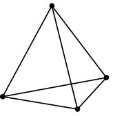	Wedge6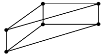	Hex8	Pyramid5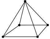


3D Quadratic Elements
Tet10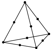	Wedge15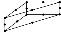	Hex20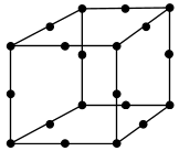	Pyramid13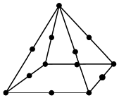

Consider an element with $n$ nodes. It is convenient to define a local coordinate system, so that the position of any point within the element can be defined using local coordinates $ξ$ .

If $ξ_{P}$ is the position vector of a point $P$ in the local coordinate system, the value of $u$ at point $P$ can then be written as:

Figure 1. EQUATION_DISPLAY

u (ξ_{P}) = N_{M} (ξ_{P}) u_{M}

(4803)

where:

the index $M = 1, ..., n$ identifies the element nodes
$u_{M} = u (ξ_{M})$ is the value of $u$ at the node $M$
$N_{M}$ is an H¹ Lagrange shape function, which determines the contribution of the nodal value $u_{M}$ to $u$
Eqn. (4803) and all following equations use Einstein notation, which implies summation over repeated indices. For example, $N_{M} u_{M} \equiv \sum_{M = 1}^{n} N_{M} u_{M}$

If $M$ and $N$ are two element nodes, with $M \neq N$ , $N_{M}$ is defined so that:

Figure 2. EQUATION_DISPLAY

\begin{matrix} N_{M} (ξ_{M}) = 1 \\ N_{M} (ξ_{N}) = 0 \end{matrix}

(4804)

The shape functions for linear tetrahedral and hexahedral elements are described below. The local coordinate system is defined using natural coordinates:

Figure 3. EQUATION_DISPLAY

ξ = {\begin{array}{l} ξ_{1} \\ ξ_{2} \\ ξ_{3} \end{array}}

(4805)

Linear Tetrahedron (Tet4): In tetrahedral elements, the local coordinates are $0 \leq \begin{matrix} ξ_{i} \end{matrix} \leq 1$ :; The nodal shape functions at a point of coordinates $({\begin{matrix} ξ \end{matrix}}_{1}, {\begin{matrix} ξ \end{matrix}}_{2}, {\begin{matrix} ξ \end{matrix}}_{3})$ are simply:; Figure 4. EQUATION_DISPLAY

$\begin{matrix} N_{1} & = & {\begin{matrix} ξ \end{matrix}}_{1} \\ N_{2} & = & {\begin{matrix} ξ \end{matrix}}_{2} \\ N_{3} & = & {\begin{matrix} ξ \end{matrix}}_{3} \\ N_{4} & = & {1 - \begin{matrix} ξ \end{matrix}}_{1} {- \begin{matrix} ξ \end{matrix}}_{2} {- \begin{matrix} ξ \end{matrix}}_{3} \end{matrix}$
(4806); which correspond to the barycentric coordinates.
Linear Hexahedron (Hex8): In hexahedral elements, the local coordinates are $- 1 \leq \begin{matrix} ξ_{i} \end{matrix} \leq 1$ :; The nodal shape functions at a point of coordinates $({\begin{matrix} ξ \end{matrix}}_{1}, {\begin{matrix} ξ \end{matrix}}_{2}, {\begin{matrix} ξ \end{matrix}}_{3})$ are:
Figure 5. EQUATION_DISPLAY

$N_{M} (ξ_{i}) = \frac{1}{8} (1 + ξ_{i M} ξ_{i}); M = 1, ..., 8$
(4807); Linear hexahedra are enriched with bubble degrees of freedom, to overcome locking phenomena. For example, the linear shape functions Eqn. (4807) do not provide enough mode shapes to approximate shear and bending in Solid Mechanics applications, causing the elements to be overly stiff. The stiffening effect worsens for high aspect ratios and skewed element shapes. To overcome locking, Simcenter STAR-CCM+ adds three additional vectors $u_{o i}$ (that is, 9 internal, or bubble, degrees of freedom) to the nodal quantities $u_{M}$ :
Figure 6. EQUATION_DISPLAY

$\begin{matrix} u (ξ_{i}) = N_{M} (ξ_{i}) u_{M} + u_{o i} (1 - ξ_{i}^{2}); & i = 1, 2, 3; M = 1, ..., 8; \end{matrix}$
(4808); The accuracy of the quadratic Hex20 element is higher than the accuracy of the linear Hex8 element with bubble functions. The Hex20 is also insensitive to high aspect ratios and skewness. Tet4 elements are stiff in bending and shear and their behavior cannot be improved with the use of bubble functions.

From Local to Global: Parametric Mapping

Local-to-global mapping between the parent domain and the global physical domain ensures continuity across adjacent elements.

Shape Function Derivatives

The derivatives of the variable $u$ with respect to the undeformed coordinates $X$ are related to the nodal quantities $u_{M}$ through:

Figure 7. EQUATION_DISPLAY

\frac{\partial u}{\partial X} = \frac{\partial N_{M}}{\partial X} u_{M}

(4809)

The derivatives of the shape functions with respect to the undeformed physical coordinates are determined from the derivatives of the shape functions with respect to the natural coordinates through:

Figure 8. EQUATION_DISPLAY

\begin{matrix} \frac{\partial N_{M}}{\partial X} = J^{- 1} \frac{\partial N_{M}}{\partial ξ} \end{matrix}

(4810)

where:

Figure 9. EQUATION_DISPLAY

\frac{\partial N_{M}}{\partial ξ} = (\begin{matrix} \frac{\partial N_{M}}{\partial ξ_{1}} \\ \frac{\partial N_{M}}{\partial ξ_{2}} \\ \frac{\partial N_{M}}{\partial ξ_{3}} \end{matrix}); \frac{\partial N_{M}}{\partial X} = (\begin{matrix} \frac{\partial N_{M}}{\partial X_{1}} \\ \frac{\partial N_{M}}{\partial X_{2}} \\ \frac{\partial N_{M}}{\partial X_{3}} \end{matrix})

(4811)

and $J^{- 1}$ is the inverse of the Jacobian transformation, $J$ :

Figure 10. EQUATION_DISPLAY

J = [\begin{matrix} \frac{\partial X_{1}}{\partial ξ_{1}} & \frac{\partial X_{1}}{\partial ξ_{2}} & \frac{\partial X_{1}}{\partial ξ_{3}} \\ \frac{\partial X_{2}}{\partial ξ_{1}} & \frac{\partial X_{2}}{\partial ξ_{2}} & \frac{\partial X_{2}}{\partial ξ_{3}} \\ \frac{\partial X_{3}}{\partial ξ_{1}} & \frac{\partial X_{3}}{\partial ξ_{2}} & \frac{\partial X_{3}}{\partial ξ_{3}} \end{matrix}]

(4812)

H1 Lagrange Shape Functions

From Local to Global: Parametric Mapping

Shape Function Derivatives

H¹ Lagrange Shape Functions