Home
Tutorials
Tutorials show you how to use Simcenter STAR-CCM+ for various applications in a step-by-step format with recommendations for setup, initialization and steps of the solution process specific to the application. Macro and simulation files are available for download for a large proportion of cases.
Aeroacoustics
The tutorials in this set illustrate various Simcenter STAR-CCM+ features for solving aeroacoustic simulations.
Lighthill Wave and Perturbed Convective Wave Modeling: Simplified HVAC Duct
Noise generated by the air handling components in heating, ventilation, and air conditioning (HVAC) systems is a large contributor to interior cabin sound levels. Investigating the sources of noise and modifying the design accordingly, leads to better and quieter systems.
Obtaining the Perturbed Convective Wave Solution
After the Lighthill Wave simulation is complete, you re-run the LES acoustics simulation using the Perturbed Convective Wave model.
Analyzing the Perturbed Convective Wave Solution
After the simulation is complete, you visualize the results of the Pertubed Convective Wave solution.

Share

Link: copied

Breadcrumb: copied

Tutorials
Tutorials show you how to use Simcenter STAR-CCM+ for various applications in a step-by-step format with recommendations for setup, initialization and steps of the solution process specific to the application. Macro and simulation files are available for download for a large proportion of cases.
- Using Tutorial Macros and Files
  Macros, input files, and final simulation files for a range of tutorials are provided as an optional download package on the Support Center website. These macros and final simulation files are provided as an aid to the written tutorials, so that you can check your final results against the downloaded files, or against a simulation that is built and run using the macros.
- Introduction
  Welcome to the Simcenter STAR-CCM+ introductory tutorial. In this tutorial, you explore the important concepts and workflow. Complete this tutorial before attempting any others.
- Foundation Tutorials
  The foundation tutorials showcase the major features of Simcenter STAR-CCM+ in a series of short tutorials.
- Geometry
  The tutorials in this set illustrate various Simcenter STAR-CCM+ features for creating and working with parts and 3D-CAD.
- Mesh
  The tutorials in this set illustrate various STAR-CCM+ features for building CFD meshes.
- Incompressible Flow
  The tutorials in this set illustrate various Simcenter STAR-CCM+ features for incompressible fluid flows as well as porosity and solution recording
- Compressible Flow
  The tutorials in this set illustrate various Simcenter STAR-CCM+ features for compressible fluid flows as well as harmonic balance.
- Heat Transfer and Radiation
  The tutorials in this set illustrate various Simcenter STAR-CCM+ features for heat transfer, radiation, and thermal comfort.
- Multiphase Flow
  The tutorials in this set illustrate various Simcenter STAR-CCM+ features for simulating multiphase fluid flow problems
- Discrete Element Method
  The tutorials in this set illustrate various Simcenter STAR-CCM+ features for simulating Discrete Element Method problems
- Motion
  The tutorials in this set illustrate various STAR-CCM+ features for simulating problems with moving geometries and meshes, dynamic fluid body interaction, and rigid body motion:
- Reacting Flow
  The tutorials in this set illustrate various Simcenter STAR-CCM+ features for simulating reacting flows such as combustion.
- Solid Stress
  The tutorials in this set illustrate various Simcenter STAR-CCM+ features for computing deformation, strain, and stresses in solid regions. They also show how such computations can be coupled to the fluid behavior in an analysis of fluid-structure interaction.
- Aeroacoustics
  The tutorials in this set illustrate various Simcenter STAR-CCM+ features for solving aeroacoustic simulations.
  - Broadband Models: Noise from a Cylinder (Preparation)
    This tutorial demonstrates how to set up aeroacoustics problems in Simcenter STAR-CCM+. The flow around a cylinder is used in the simulation to describe the required steps.
  - DES and FW-H On-The-Fly: Noise from a Cylinder (Unsteady Analysis)
    In the previous section of this tutorial, you completed the steady-state analysis runs for qualifying the volume mesh. In this section, continuing from the previous simulation file, you set up the final transient run for an unsteady analysis of the near field and an FW-H analysis of the far field.
  - Ffowcs Williams-Hawkings: Sound Propagation
    This tutorial compares the Post FW-H model with the FW-H On-The-Fly model.
  - Signal Post-Processing: FFT and Wavenumber
    Several further analyses are possible using the simulation history file from the earlier tutorial, DES and FW-H On-The-Fly: Noise from a Cylinder (Unsteady Analysis). These analyses are covered in this tutorial.
  - Acoustic Wave Modeling: Noise from a Cylinder
    This tutorial demonstrates how to set up an acoustic wave simulation in Simcenter STAR-CCM+. The flow around a cylinder is used in the simulation to describe the required steps.
  - Lighthill Wave and Perturbed Convective Wave Modeling: Simplified HVAC Duct
    Noise generated by the air handling components in heating, ventilation, and air conditioning (HVAC) systems is a large contributor to interior cabin sound levels. Investigating the sources of noise and modifying the design accordingly, leads to better and quieter systems.
    - Prerequisites
      The instructions in the Lighthill Wave and Perturbed Convective Wave Modeling: Simplified HVAC Duct tutorial assume that you are already familiar with certain techniques in Simcenter STAR-CCM+.
    - Loading the Starting Simulation File
      You start this tutorial by loading a simulation file that includes the geometry of the HVAC duct, mesh operations that create the flow domain and generate a trimmed mesh, physics continua for a steady RANS and an unsteady LES simulation, and regions including boundary types. Two-sequences of simulation operations are set up to automate the processes of running a RANS simulation followed by an LES acoustics simulation.
    - Running the RANS Simulation
      You generate the mesh und run the RANS simulation using the pre-defined simulation operation 01_RANS.
    - Setting the Appropriate Cell Size and Time-Step Size for the LES Acoustics Simulation
      Based on the RANS simulation results and the frequency of the acoustic waves to be resolved, you determine the cell size and the time-step size for the LES acoustics simulation.
    - Enhancing the LES Solution Accuracy and Convergence Rate
      High-order temporal discretization schemes give faster unsteady solutions by allowing the use of larger time-steps while also being more accurate than lower-order schemes. Therefore, you use a second-order temporal discretization scheme. Additionally, you reduce gradients limiting, which allows higher gradient variations in the flow field.
    - Obtaining the Lighthill Wave Solution
      Starting from the steady RANS simulation, you perform an unsteady LES acoustics simulation using the Lighthill Wave model.
    - Obtaining the Perturbed Convective Wave Solution
      After the Lighthill Wave simulation is complete, you re-run the LES acoustics simulation using the Perturbed Convective Wave model.
      - Setting Up the Perturbed Convective Wave Model
        For the Perturbed Convective Wave simulation, you replace the Lighthill Wave model in the LES physics continuum with the Perturbed Convective Wave model.
      - Preparing Scenes and Plots for the Acoustics Analysis
        To analyze the Perturbed Convective Wave solution, you set up plots that display the acoustic pressure and the pressure perturbation over time at the microphone and at the pressure transducer. Additionally, you prepare visualization of the acoustic pressure within the flow domain.
      - Running the LES Simulation for the Perturbed Convective Wave Solution
        The setup for the Perturbed Convective Wave simulation is now complete. To run the simulation, you re-play the simulation operation 02_LES.
      - Analyzing the Perturbed Convective Wave Solution
        After the simulation is complete, you visualize the results of the Pertubed Convective Wave solution.
    - Comparing Results Using Spectral Analyses
      To compare the Lighthill Wave solution with the Perturbed Convective Wave solution, you perform spectral analyses at the microphone and the pressure transducer. Using pre-defined Point Time Fourier Transforms, you transform the time signals (Lighthill pressure, acoustic pressure, and pressure perturbation) to the frequency domain. You display the results using monitor plots.
  - Sponge Layer Modeling: Simplified Tailpipe
    Unsteady aeroacoustics simulations require effective non-reflective boundary conditions to prevent spurious reflected acoustic waves from the boundaries of the computational domain interfering with the aeroacoustic results.
- Electromagnetism
  The following tutorials illustrate features for solving problems that involve electromagnetic fields.
- Electrochemistry
  The following tutorial demonstrates chemical reactions induced by an electrical current.
- Battery
  The tutorials in this set illustrate various Simcenter STAR-CCM+ features for setting up a battery model:
- Automation
  The tutorials in this set illustrate various Simcenter STAR-CCM+ automation and macro features.
- Design Exploration
  The tutorials in this set illustrate various features for running design exploration studies in Design Manager.
- Coupling with CAE Codes
  The tutorials in this set illustrate various Simcenter STAR-CCM+ features for coupling with CAE codes:
- Analysis Methods
  The tutorials in this set illustrate various Simcenter STAR-CCM+ features for analysing and visualizing simulation data.
- Simcenter STAR-CCM+ In-cylinder
  The tutorials in this set illustrate features for simulating internal combustion engines in Simcenter STAR-CCM+ using the dedicated add-on Simcenter STAR-CCM+ In-cylinder.

Analyzing the Perturbed Convective Wave Solution

After the simulation is complete, you visualize the results of the Pertubed Convective Wave solution.

To analyze the Perturbed Convective Wave solution:

Examine the plots that display the acoustic pressure and the pressure perturbation at the microphone and at the pressure transducer by clicking through the Microphone: Acoustic Pressure and Pressure Perturbation Monitors Plot and Pressure Transducer: Acoustic Pressure and Pressure Perturbation Monitors Plot tabs in the Graphics window.
The following plots display the results after the run:

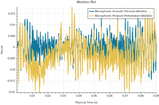
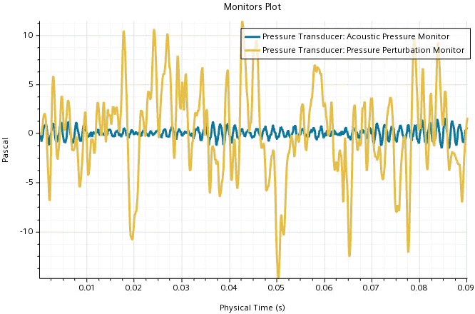
At the microphone, the acoustic pressure and the pressure perturbation are of the same order of magnitude. As the pressure perturbation represents the sum of acoustic and hydrodynamic pressure, this indicates that the hydrodynamic pressure in this region is less relevant.

At the pressure transducer, the pressure perturbation shows higher amplitudes than the acoustic pressure. Here, the hydrodynamic pressure contribution is dominant.
To examine the acoustic pressure, click on the Acoustic Pressure tab.
The following screenshot shows the acoustic pressure within the flow domain:

Similar to the Lighthill pressure time derivative as displayed in Analysing the Lighthill Wave Solution, this scene shows how the acoustic pressure radiates from the HVAC duct into the test chamber. However, the acoustic pressure as solved by the Perturbed Convective Wave model shows no turbulent structures. This solution field gives direct insight into the noise field without any hydrodynamic perturbations.
Save the simulation.