AMUSIG Breakup and Coalescence

The Simcenter STAR-CCM+ breakup and coalescence models for AMUSIG are not suitable for particulate flow. However, you can use AMUSIG to model the size distribution of solid particle phases in a particulate flow: use your own understanding and knowledge of coalescence and breakup phenomena for the application of interest to calibrate power law coalescence and breakup models as appropriate.

A set of models is available for describing breakup and coalescence processes for different applications:

• The model of Luo ([513]), and O'Rourke ([524]) are provided for turbulent coalescence.
• The model of Tsouris and Tavlarides ([515]), the model of Martinez-Bazan ([515]), the model of Kocamustafaogullari ([515]) and the model of Coulaloglou and Eskin ([456]) are provided for break-up in turbulent liquid/liquid and bubbly flows.
• Shear-induced breakup and coalescence models are provided for laminar flows.
• Constant and power-law models are also implemented for testing and demonstration purposes, and to provide some user-specified modeling.

The Coalescence Rate model has submodels for Collision Rate and Coalescence Efficiency. The Breakup Rate model has submodels for Breakage Rate and Fragments Particle Size Distribution, which defines a removal term for particles of a given size. All of the rate models have an overall calibration constant which you can adjust to suit your requirements. The Critical Weber number is an adjustable parameter that is relevant for the breakup rate models.

A single size-group is sufficient for modeling hydrostatic expansion of dilute bubbles rising in a deep tank or column. However, for a meaningful collision/breakup study, a minimum of three groups is recommended. The adaptivity of the AMUSIG model allows you to investigate significant and rapid changes of particle size with a few groups. Increasing the number of groups should lead to resolution-independent results, in a manner similar to mesh refinement. Computational cost sets the practical upper limit on the number of size-groups.

Laminar and Turbulent Breakup Models

The breakup process is modeled in two parts, a breakage rate and a fragments particle size distribution. The breakup rate has a dimension of time^-1, so the probability that a single particle is broken within the time span $\mathrm{dt}$ is (breakup rate) $\mathrm{dt}$ . The fragment size distribution is dimensionless. It determines how many fragments are created, and the distribution of the fragments.

Power Law Breakage Rate

This model applies to both turbulent breakup and laminar breakup. The power law breakage rate model describes how quickly a particle of a given size can be broken. This model is a generic model with adjustable parameters for the breakage rate multiplier $K_B$ of number density at some particle size $d$ scaled by a characteristic diameter $d_0$ .

$$K_B\left(d\right)=C{\left(\frac{d}{d_0}\right)}^a$$

(2244)

Since the product of $K_B$ and number density is a rate in events per second per $m^3$ , the calibration constant $C$ has dimensions of per second.

This breakage rate enters the conservation equations as any other breakage rate:

$$\frac{Dn}{Dt}=-(\mathrm{breakage}\mathrm{rate})*n$$

(2245)

where:

• ${\epsilon }_f$ is the turbulent dissipation rate of the continuous phase.
• $d_p$ is the diameter of the particle.
• $\mathrm{We}$ is the Weber number.
• ${\mathrm{We}}_{\mathrm{cr}}$ is the critical Weber number. It determines the size of the particle that can survive the given intensity of turbulence. A high value of ${\mathrm{We}}_{\mathrm{cr}}$ implies that the breakup is weak.
• $C_g$ is a calibration constant that can be used to adjust the breakup time scale.

For turbulent flows, the Weber number is given by:

The correction factor ${\left(\frac{{\rho }_p}{{\rho }_f}\right)}^{1/3}$ implies that bubbles can survive stronger turbulence than droplets [501]. This correction can overestimate the diameter of the bubbles. However, you can increase the breakup rate by decreasing the critical Weber number.

Martinez-Bazan

For the function $f$ in Eqn. (2246), the Martinez-Bazan model assumes a square root shape. The Martinez-Bazan model implies that there is a minimum diameter below which no breakup occurs.

Tsouris and Tavlarides

For the function $f$ in Eqn. (2246), the Tsouris and Tavlarides model uses an exponent. The Tsouris and Tavlarides model predicts that any droplet can be broken (there is no minimum diameter), but the breakup probability decreases exponentially with droplet diameter.

Coulagloglou and Eskin

The Coulaloglou and Eskin model predicts a broader size distribution than the other two models.

Kocamustafaogullari

The Kocamustafaogullari model is suitable for modeling the break-up of liquid droplets in continuous gas. The model accounts for the deformation resisted by surface tension and viscous forces inside the liquid droplet. The characteristic measures of this behavior are the Weber and Ohnesorge numbers.

For laminar flows, the breakup of droplets is controlled by the capillary number. The capillary number is the ratio of the viscous shear stress that tries to deform and break up the droplet, and the capillary pressure that preserves the spherical shape of the droplet, and is given by:

where:

The laminar breakup models assume that there is a critical value ${Ca}_{cr}$ such that for ${Ca<Ca}_{cr}$ the breakup rate is small or zero and for ${Ca>Ca}_{cr}$ the breakup rate is strong. This critical capillary number can be defined as a function of the viscosity ratio $\lambda =\frac{{\mu }_d}{{\mu }_c}$ , where ${\mu }_d$ is the dynamic viscosity of the dispersed phase:

where:

For the laminar breakup models, the breakup rate has the following structure:

where:

The difference between the laminar breakup models is in the function $f$ in Eqn. (2250):

Cristini

The Cristini model defines $f$ as ([445]):

$$f=\{\begin{array}{cc}\sqrt{\frac{1}{\mathrm{\Phi }-1}}& ,\mathrm{\Phi }<1\\ 0& ,\mathrm{\Phi }\ge 1\end{array}$$

(2252)

Tsouris and Tavlarides

For the Tsouris and Tavlarides Shear model, the breakup probability decreases exponentially with droplet diameter. The function $f$ is given as:

$$f=\exp (-\mathrm{\Phi })$$

(2253)

Coulaloglou and Eskin

The Coulaloglou and Eskin Shear model defines $f$ as:

$$f=erfc\left(\sqrt{\mathrm{\Phi }}\right)\sqrt{\frac{4\mathrm{\Phi }}{\pi }}\exp (-\mathrm{\Phi })$$

(2254)

where $erfc$ is the complementary error function.

Kocamustafaogullari

The Kocamustafaogullari model is based on the stochastic secondary droplet (SSD) model, which assumes

the following instantaneous breakup rate of a droplet:

$$\mathrm{B}\mathrm{r}\mathrm{e}\mathrm{a}\mathrm{k}\mathrm{u}\mathrm{p}\mathrm{}\mathrm{R}\mathrm{a}\mathrm{t}\mathrm{e}=\{\begin{array}{cc}0& ,We\le {We}_{cr}\\ B_1\sqrt{\frac{{\rho }_g}{{\rho }_l}}\frac{w}{Dp}& ,We<{We}_{cr}\end{array}$$

(2255)

where:

• ${We}_{cr}$ is the critical Weber number. The default value is 12.
• $B_1$ is a parameter regulating the speed of breakup. Large values signify that breakup occurs later. The default value is $2\sqrt{3}$ .
• ${\rho }_l$ is the density of the liquid.
• $Dp$ is the droplet diameter.
• ${\rho }_g$ is the density of the gas.
• $w_t$ is the turbulent slip velocity of the droplet through the continuous phase.

Kocamustafaogullari ([488]) correlated the experimental data for droplet size distribution in annular flows by using Levich [501] formulations for the equation of motion of a droplet in a turbulent flow:

$$\frac{{\rho }_l{D}_p^3}{6}\frac{{du}_l^{\prime }}{dt}=-C_D{\rho }_g\frac{\pi D_p^2}{4}|u_l^{\prime }-u_g^{\prime }|(u_l^{\prime }-u_g^{\prime })$$

(2256)

where $u_l^{\prime }$ and $u_g^{\prime }$ are the fluctuating velocity of liquid and gas, respectively. Assuming that the drag coefficient is $C_d=0.5$ Eqn. (2256) then is rearranged into:

$${\rho }_l(\frac{{dw}_t}{dt}+0.75\frac{{\rho }_g}{{\rho }_l}\frac{w_t}{Dp}{w}_t)=-{\rho }_l\frac{d{u}_g^{\prime }}{dt}$$

(2257)

Using Kolmogorov scaling and based on their experiments with non-buoyant particles, Kuboi [491]estimated the fluctuating component of the gas velocity at a scale λ as:

$$|{u_g^{\prime }|}^2=2{\left({ϵ}_g\lambda \right)}^{2/3}$$

(2258)

The acceleration in a gas vortex of size λ can be estimated as:

$$\frac{d{u}_g^{\prime }}{dt}\sim 2\frac{{\left({ϵ}_g\lambda \right)}^{1/3}}{\lambda },\frac{d{w}_t}{dt}\sim \frac{\langle w_t\rangle }{\lambda }$$

(2259)

Substituting Eqn. (2258) in Eqn. (2256) yields:

$$\langle w_t^2\rangle =\frac{2{\left({ϵ}_g\lambda \right)}^{2/3}}{1+0.75\frac{{\rho }_g}{{\rho }_l}\frac{\lambda }{Dp}}$$

(2260)

Eqn. (2260) attains its maximum value at:

$$\begin{gathered} {\lambda }_{\max }=\frac{8}{3}\frac{{\rho }_l}{{\rho }_g}Dp \\ {\langle {w_t}^2\rangle }_{\max }=\frac{4}{3}{\left(\frac{{\rho }_l{ϵ}_{g}Dp}{3{\rho }_g}\right)}^{2/3} \end{gathered}$$

(2261)

The non-dimensional slip velocity is $w=\sqrt{\frac{\sigma }{{\rho }_{g}Dp}}W,\langle w\rangle =\sqrt{\frac{\sigma }{{\rho }_{g}Dp}}U,\langle w_t\rangle =\sqrt{\frac{\sigma }{{\rho }_{g}Dp}}r$ , where $W$ and $U$ are the non-dimensional mean and fluctuating slip velocity. The normalized distribution is given as :

$$f\left(w\right)\left(W\right)=\sqrt{\frac{\beta }{\pi }}\frac{W}{U}[\exp (-\beta {(W-U)}^2)-\exp (-\beta {(W+U)}^2\left)\right]$$

(2262)

where $\beta =\frac{3}{2\left({We}_t\right)}$

For zero mean slip, Eqn. (2262) slip reduces to:

(2263)

$$f\left(w\right)\left(W\right)=4\sqrt{\frac{{\beta }^3}{\pi }}{W}^2[\exp (-\beta W^2)$$

(2264)

Kocamustafaogullari has shown that using the characteristic slip velocity given by Eqn. (2256) to Eqn. (2261), it is possible to correlate the available experimental data. Eqn. (2255) is then averaged over all possible realizations of the slip velocity:

$$\mathrm{B}\mathrm{r}\mathrm{e}\mathrm{a}\mathrm{k}\mathrm{u}\mathrm{p}\mathrm{}\mathrm{R}\mathrm{a}\mathrm{t}\mathrm{e}=B_1\{\begin{array}{cc}{\left(\frac{8}{3\pi }\frac{{\rho }_g}{{\rho }_l}\frac{{\langle w}_t^2\rangle }{{Dp}^2}\right)}^{1/2}(1+\beta {We}_{cr})\exp (-\beta {We}_{cr})& ,U=0\\ \sqrt{\frac{{\rho }_g}{{\rho }_l}}\frac{\langle w\rangle }{Dp}& ,U\gg \sqrt{{We}_{cr}}\end{array}$$

(2266)

(2265)

Effect of the Liquid Viscosity

The effect of the liquid viscosity on the breakup rate is characterized by the Ohnesorge number [470]:

$$\mathrm{Oh}=\frac{{\mu }_l}{\sqrt{{\rho }_l{D}_p\sigma }}$$

(2267)

where ${\mu }_l$ is the liquid viscosity and $\sigma$ is the surface tension of the liquid.

To account for the enhanced stability of more viscous droplets, a correlation for the critical Weber and Ohnesorge numbers is defined as:

$${We}_{cr}={We}_{cr|O_h=0}\cdot (1+a{Oh}^b)$$

(2268)

where $a$ and $b$ are constants, derived by Gelfand in [464].

Coalescence Models

The coalescence process is modeled in two parts, a collision rate and a coalescence efficiency.

Turbulent Collision Rate

Applies to turbulent coalescence only. The coalescence rate is a product of collision rate and coalescence efficiency. The turbulent collision rate is calculated as the probability of collision of two spheres with diameters $d_1$ and $d_2$ moving with random relative velocity $v={\left({ϵ}_f\frac{d_1+d_2}{2}\right)}^{1/3}$ .

The model has no fitting parameters, apart from those in the coalescence efficiency submodels.

Luo Coalescence Efficiency

The Luo coalescence efficiency model ([513]) assumes that the coalescence happens when the contact time $t_{contact}$ is bigger than $t_{rupture}$ — the time that is needed to break the liquid film separating two bubbles:

$$\mathrm{C}\mathrm{o}\mathrm{a}\mathrm{l}\mathrm{e}\mathrm{s}\mathrm{c}\mathrm{e}\mathrm{n}\mathrm{c}\mathrm{e}\mathrm{}\mathrm{E}\mathrm{f}\mathrm{f}\mathrm{i}\mathrm{c}\mathrm{i}\mathrm{e}\mathrm{n}\mathrm{c}\mathrm{y}\sim \exp (-C\frac{t_{rupture}}{t_{contact}})$$

(2269)

where $C$ is the only calibration constant of the model. High $C$ means that there is no coalescence; the default value is $C=1$ .

O'Rourke Coalescence Efficiency

The O'Rourke coalescence efficiency model ([524]) detects collisions of the liquid droplets in a continuous gas phase. The colliding liquid droplets undergo a chaotic motion due to the turbulent fluctuations of the continuous phase. The collision outcome is controlled by the collision Weber number:

$${\text{We}}_{\text{coll}}=\frac{{\rho }_l{\left(w\right)}^2(r_1+r_2)}{2\sigma }$$

(2270)

where:

• $r_i,i=1,2,\mathrm{..}$ is the droplet radius.
• $\sigma =\frac{1}{2}({\sigma }_1+{\sigma }_2)$ is the average surface tension of droplets 1 and 2.
• ${\rho }_l=\frac{1}{2}({\rho }_1+{\rho }_2)$ is the average density.
• $w$ is the relative velocity of two droplets, due to only the turbulent fluctuations as computed in Eqn. (2261).

The outcome of a collision is based on the impact parameter $B$ and the collision Weber number $\text{We}$ . The collision Weber number ${\text{We}}_{\text{coll}}$ is calculated by Eqn. (2270) for each pair of interacting droplets. The collision efficiency $E$ is defined as the probability of obtaining a given outcome ( $E=B\cdot B$ ).

The droplet size ratio $\gamma$ is:

$$\gamma =\frac{r_2}{r_1},r_2>r_1$$

(2271)

The droplet diameter ratio correction is defined as:

$$g\left(\gamma \right)=a_3{\gamma }^3+a_2{\gamma }^2+a_1\gamma +a_0$$

(2272)

where $\gamma$ is the droplet size ratio. The default values for the constants are:

• $a_3=2.4$
• $a_2=-5.76$
• $a_1=6.48$
• $a_0=0$

For the given value of the collision velocity $w$ , the probabilities of no bounce and no separation reduce to these formulations:

$$E_{noseparation}=\text{min}[1.0,\frac{g\left(\gamma \right)}{We}]$$

(2273)

and

$$E_{nobounce}=\text{min}[1.0,{\left(\frac{We}{g\left(\gamma \right)}\right)}^{\frac{1}{3}}]$$

(2274)

The product of Eqn. (2273) and Eqn. (2274) is the probability of the coalescence:

$$E_{coal}=\text{min}(\frac{g\left(\gamma \right)}{We},{\left(\frac{We}{g\left(\gamma \right)}\right)}^{\frac{1}{3}})$$

(2275)

The coalescence efficiency is then obtained by averaging Eqn. (2274) with the breakup distribution function Eqn. (2264) :

$${\lambda }_c=\frac{1}{3\sqrt{\pi }{\mathrm{\Phi }}^{1/3}}\left[5\mathrm{\Gamma }\right(\frac{5}{6},\mathrm{\Phi })-6{\mathrm{\Phi }}^{5/6}\cdot \exp (-\mathrm{\Phi }\left)\right]+2\mathrm{\Phi }\cdot erfc\left(\sqrt{\mathrm{\Phi }}\right)$$

(2276)

where $\mathrm{\Gamma }$ is the incomplete gamma function, and $\mathrm{\Phi }$ is defined as:

$$\mathrm{\Phi }=\frac{3g\gamma }{8W_{et}}$$

(2277)

where

$${\mathrm{W}\mathrm{e}}_t=\frac{{\rho }_l\langle w_t^2\rangle (r_1+r_2)}{2\sigma }$$

(2278)

The coalescence efficiency map is plotted below.

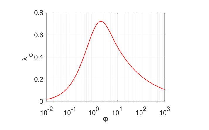
The maximum efficiency is reached at $\mathrm{\Phi }=1$ . The region for $\mathrm{\Phi }\ll 1$ corresponds to high kinetic energy of collision due to surface tension instabilities. In this region, the droplet and the coalescence efficiency are low. The coalescence efficiency decays for $\mathrm{\Phi }\gg 1$ , which is a result of a large droplet size ratio between the two droplets ( $g\left(\gamma \right)\gg 1$ ) or low droplet relative velocity.

Film Drainage Coalescence Efficiency

The Film Drainage coalescence efficiency model is a generic model that is compatible with any collision rate model.

$$\mathrm{C}\mathrm{o}\mathrm{a}\mathrm{l}\mathrm{e}\mathrm{s}\mathrm{c}\mathrm{e}\mathrm{n}\mathrm{c}\mathrm{e}\mathrm{}\mathrm{E}\mathrm{f}\mathrm{f}\mathrm{i}\mathrm{c}\mathrm{i}\mathrm{e}\mathrm{n}\mathrm{c}\mathrm{y}\sim \exp (-C\frac{{\mathrm{W}\mathrm{e}}^m}{{\mathrm{Re}}^n})$$

(2279)

where $\mathrm{W}\mathrm{e}$ is the collision Weber number:

$$\mathrm{W}\mathrm{e}=\frac{\rho U_c^2{d}_{eff}}{\sigma }$$

(2280)

and $\mathrm{Re}$ is the collision Reynolds number:

$$\mathrm{Re}=\frac{\rho U_c{d}_{eff}}{\mu }$$

(2281)

The velocity of collision $U_c$ is provided by the collision rate model. $d_{eff}$ is the effective diameter of the colliding droplets or bubbles.

Laminar Collision Rate

For the laminar collision rate, the relative velocity of two spheres is due to the mean shear rate:

$$v=\dot{S}\frac{d_1+d_2}{2}$$

(2282)

Enhanced Power Law Collision Rate

This collision rate model applies to both Turbulent Coalescence and Laminar Coalescence.

Enhanced Power Law Collision Rate with its adjustable parameters allows investigation of alternative coagulation kernels $K$ between particles of two sizes $d_1$ and $d_2$ , scaled by characteristic diameter $d_0$ .

$$K(d_1,d_2)=C{[{\left(\frac{d_1}{d_0}\right)}^a+{\left(\frac{d_2}{d_0}\right)}^a]}^b{[{\left(\frac{d_1}{d_0}\right)}^c+{\left(\frac{d_2}{d_0}\right)}^c]}^d$$

(2283)

Since the product of the kernel with the number densities of the two colliding sizes is a rate in events per second per $m^3$ , the calibration constant $C$ has dimensions of $m^3$ per second.