Sampling Methods for Robustness and Reliability Studies

In a Robustness and Reliability study, all the input parameters are continuous. Distribution values are specified for each parameter and the sampling method chooses values according to the specified distributions.

In the input parameter properties, you specify Distribution Value for each parameter. For more details, refer to: Distribution Value (Robustness and Reliability Study).

When distribution values are set, the associated Probability Density Function (PDF) $f (x)$ and Cumulative Distribution Function (CDF) $F (x)$ are fully determined for this input parameter.

The sample points (values of this input parameter) are chosen by mapping random sample points $u^{(i)}$ between 0 and 1 on the reverse function of the CDF, $F^{- 1} (x)$ :

Figure 1. EQUATION_DISPLAY

x^{(i)} = F^{- 1} (u^{(i)})

(5142)

where $u^{(i)} \in [0, 1]$ are random samples from 0 to 1, which are generated by the computer.

$x^{(i)}$ are the resulting input parameter values which match the desired distribution.

From the statistics point of view, the values are more likely to come from the portion of the range for which the CDF is steeper.

For a Robustness and Reliability study, the following sampling methods are available:

Latin Hypercube Sampling
Monte Carlo Sampling

Latin Hypercube Sampling

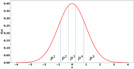
For m Designs to Run (sample size), the Latin Hypercube sampling divides the distribution function $f (x)$ into $m$ segments with equal area and picks one value for each segment. An example of one input parameter with normal distribution and 5 Designs to Run is shown below:

The mapping step from $u^{(i)} \in [0, 1]$ to $x^{(i)}$ using the CDF $F (x)$ is shown below:

The $i^{t h}$ sample point $u^{(i)}$ is chosen to be between $\frac{i - 1}{m}$ and $\frac{i}{m}$ .

In general, for Latin Hypercube Sampling, $u^{(1)} \in [0, \frac{1}{m}], u^{(2)} \in (\frac{1}{m}, \frac{2}{m}], \dots, u^{(m)} \in (\frac{m - 1}{m}, 1]$ .

In the example above, for which $m = 5$ , the sample point $x^{(4)}$ for the fourth segment is generated by the value $u^{(4)} \in (0.6, 0.8]$ .

The following plots demonstrate the percentage of designs falling within each segment for different sample sizes:

Monte Carlo Sampling

The Monte Carlo sampling method generates independent random sample points from the distribution function without taking into account the previously generated points.

The mapping step of the Monte Carlo sampling method is shown below:

Each value $u^{(i)} \in [0, 1]$ is an independent random sample from 0 to 1.

Due to the characteristic of the Monte Carlo sampling method, a large sample size is required.

The following plots demonstrate the percentage of designs falling within each segment for different sample sizes: