Validating the Results
Compare the results against experimental data.
The S-Gamma and non-S-Gamma solutions are validated against experimental data. The experimental data has been provided in two comma-separated values (.csv) files. You import this data in the simulation as tables.
To validate the results:
- Right-click the node and select .
- In the Open dialog, navigate to the multiphaseFlow folder of the downloaded tutorial files, and multi-select the files vAir.csv and voidFraction.csv.
- Click Open.
-
Using the same technique, import the .csv files that you exported in the first part of this tutorial:
- nonSGamma_vAir.csv
- nonSGamma_voidFraction.csv.
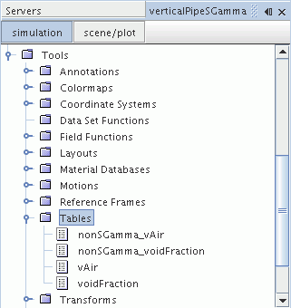
The updated Tables node is shown below.
The tabular data is now added to the plots, starting with the Volume Fraction of Air plot:
- Select the node.
- Right-click the Data Series node and select Add Data.
- In the Add Data Providers to Plot window, select voidFraction.
-
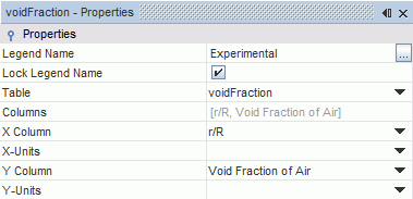
Select the
node and do the following:
- Set the Legend Name to Experimental.
- Set the Table to voidFraction using the drop-down menu.
- Set the X Column to r/R.
- Set the Y Column to Void Fraction of Air.
-
Select the
node and do the following:
- Set the Color to Black.
- Set the Shape to Filled Circle.
Add the non-S-Gamma data set to the plot.
-
Add a tabular data set as described previously and select the
NonSGamma_voidFraction data provider.
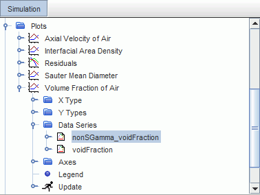
- Select the node.
Do the following:
- Set the Legend Name to NonSGamma.
- Set the Table to nonSGamma_voidFraction using the drop-down menu.
- Set the X Column to Line Probe: Normalized Radial Position.
- Set the Y Column to Line Probe: Volume Fraction of Air.
-
Select the
node and do the following:
- Set the Color to a color of your choice. In this tutorial, Blue is used for the non-S-Gamma data set.
- Set the Style to Solid.
- Select the node and set the Color to Blue.
Rename the original data set for this simulation.
- Select the node and set the Legend Name to S-Gamma.
Set the line type for the S-Gamma data set to Solid:
- Select the node and set the Style to Solid.
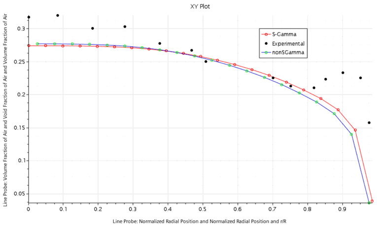
The Volume Fraction of Air plot appears as shown below.
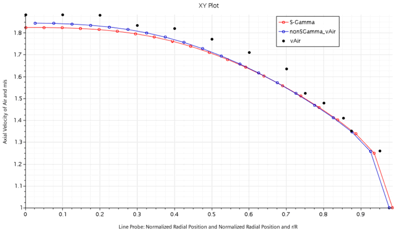
Add the remaining data sets to the Axial Velocity of Air plot using the techniques described above.
- Add the two data sets to the Data Series node in the Axial Velocity of Air plot. Rename one of the data sets to vAir and the other to NonSGamma_vAir.
- Right-click the vAir data set node and select Edit.
-
In the
Edit dialog, set the properties as shown in the table below.
Node
Value
Table
vAir
X Column
r/R
Y Column
Axial Velocity of Air
Black
Filled Circle
Do the same for the NonSGamma data set.
- Right-click the NonSGamma_vAir data set node and select Edit.
-
In the
Edit dialog, set the properties as shown in the table below.
Node
Value
Table
nonSGamma_vAir
X Column
Line Probe: Normalized Radial Position
Y Column
Line Probe: Velocity of Air[i]
Blue
Solid
Blue
Rename the original data set for this simulation:
- Select the node and set the Legend Name to S-Gamma.
Set the line type for the S-Gamma data set to Solid:
- Select the node and set the Style to Solid.
The Axial Velocity of Air plot is shown below.
- Save the simulation.