Setting Up the Plots
Create a plot to view the simulation results.
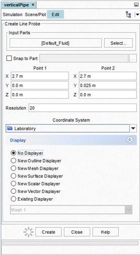
A line probe is created and used to extract data across the radius of the bubble column. When creating a derived part, Simcenter STAR-CCM+ automatically uses the active scene to display a preview of the part.
To set up the plots:
- Right-click the Derived Parts node and select .
-
In the Create Line Probe panel, do the
following:
The x-axis in the plots indicates the radial position of the data points in the pipe. For convenience, use the normalized radial position (r/R), which can be specified using a field function:
- Right-click the node and select .
- Rename the User Field Function 1 node to Normalized Radial Position.
- Set the Function Name to Normalized Radial Position.
-
Set the Definition to
$$Position(@CoordinateSystem("Laboratory"))[1]/0.0254
Note Two dollar symbols ($$) are used when referencing a position field function. 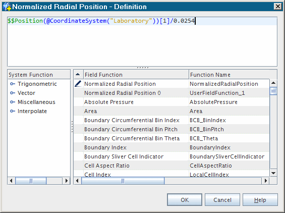
The plot can now be created.
-
Click
 (Create/Open Plots) in the
Plot toolbar and select XY
Plot.
- Rename the node to Volume Fraction of Air.
-
In the Parts property, click
 (Custom
Editor).
In the Volume Fraction of Air - Parts dialog, select .
 - Select the node and set the Data Type to Scalar.
-
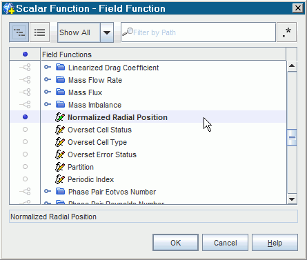
Select the node and set the Field Function
property to Normalized Radial Position.
-
Select the node.

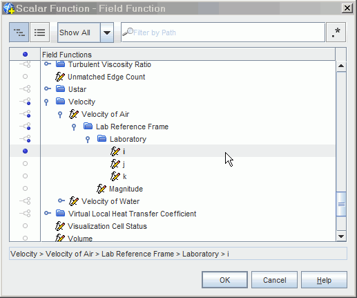
- Set the Field Function property to .
The remaining plot shares many properties with the first plot, so you can copy and paste the original plot to create the remaining plot and change some of the properties as necessary:
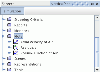
- Right-click the node and select Copy, then right-click the Plots node and select Paste.
- Rename the new plot Axial Velocity of Air.
-
Right-click the Plots node and select
Refresh.
-
Select the node and set the Field Function to .
- To open the plots, right-click the Plots node and select Open All Plots. Use the tabs at the top of the Graphics window to display each plot.
- Save the simulation.
