Importing 1D Data as Table and Specifying the Boundary Conditions
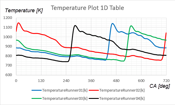
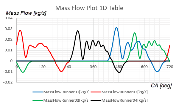
The exhaust manifold of this tutorial is part of a four-stroke four cylinder engine. Within one engine cycle the crankshaft completes two revolutions (720 deg). Mass flows and temperatures passing through exhaust runners and the pressure at the manifold outlet are time-dependent (crank angle dependent) quantities. These quantities are obtained from a 1D engine block simulation for one engine cycle.
-
To import the boundary conditions table:
- Right-click the node and select .
- In the dialog select 1D_table.csv from the heatTransferAndRadiation folder of the downloaded tutorial files and click Open.
-
Create a report that returns the current time for the fluid solution:
To apply boundary conditions that interpolate the 1D table, you use
the
interpolateTablePeriodic function. The function is set to interpolate
values based on the relative time elapsed within the current fluid engine cycle,
irrespective of how many engine cycles have already been completed. - Expand the node and multi-select the nodes, runner01, runner02, runner03, runner04, and outlet. Right-click one of the nodes and select Edit.
-
Within the Multiple Objects dialog, click
Expand/Contract Tree followed by Expand/Contract
Values. For each boundary, keep the Method for the following [physics values]
as Constant and assign their values
as shown in the table:
Boundary Physics Values Node Properties Setting runner01 Mass Flow Rate Value interpolateTablePeriodic(@Table("1D_table"),"time", LINEAR, "MassFlowRunner01[kg/s]",${PhysicalTimeFluid(s)Report}, ${FluidCycleLength(s)}) Total Temperature Value interpolateTablePeriodic(@Table("1D_table"),"time", LINEAR, "TemperatureRunner01[k]",${PhysicalTimeFluid(s)Report}, ${FluidCycleLength(s)}) runner02 Mass Flow Rate Value interpolateTablePeriodic(@Table("1D_table"),"time", LINEAR, "MassFlowRunner02[kg/s]",${PhysicalTimeFluid(s)Report}, ${FluidCycleLength(s)}) Total Temperature Value interpolateTablePeriodic(@Table("1D_table"),"time", LINEAR, "TemperatureRunner02[k]",${PhysicalTimeFluid(s)Report}, ${FluidCycleLength(s)}) runner03 Mass Flow Rate Value interpolateTablePeriodic(@Table("1D_table"),"time", LINEAR, "MassFlowRunner03[kg/s]",${PhysicalTimeFluid(s)Report}, ${FluidCycleLength(s)}) Total Temperature Value interpolateTablePeriodic(@Table("1D_table"),"time", LINEAR, "TemperatureRunner03[k]",${PhysicalTimeFluid(s)Report}, ${FluidCycleLength(s)}) runner04 Mass Flow Rate Value interpolateTablePeriodic(@Table("1D_table"),"time", LINEAR, "MassFlowRunner04[kg/s]",${PhysicalTimeFluid(s)Report}, ${FluidCycleLength(s)}) Total Temperature Value interpolateTablePeriodic(@Table("1D_table"),"time", LINEAR, "TemperatureRunner04[k]",${PhysicalTimeFluid(s)Report}, ${FluidCycleLength(s)}) outlet Pressure Value interpolateTablePeriodic(@Table("1D_table"),"time", LINEAR, "OutletPressure[Pa]",${PhysicalTimeFluid(s)Report}, ${FluidCycleLength(s)}) Static Temperature Value interpolateTablePeriodic(@Table("1D_table"),"time", LINEAR, "OutletTemperature[k]",${PhysicalTimeFluid(s)Report}, ${FluidCycleLength(s)})