Viscous Regime Models Reference

The Viscous Regime models allow you to model inviscid, laminar, or turbulent flows.

Model Names and Abbreviations Inviscid INV
Laminar LAM
Turbulent TRB
Provided By [physics continuum] > Models > Viscous Regime
Example Node Path Continua > Physics 1 > Models > Laminar
Requires
  • Material: one of Gas, Liquid, Multiphase, Multi-Component Gas, Multi-Component Liquid
  • Flow: any
Activates Physics Models Optional Models: Maxwell Slip (LAM)
Material Properties
  • Dynamic Viscosity (LAM, TRB)
See Material Properties.
Boundary Inputs See Boundary Settings.
Field Functions
  • Dynamic Viscosity (LAM, TRB)
  • Effective Viscosity (LAM, TRB)
  • Skin Friction Coefficient (LAM, TRB)
  • Wall Shear Stress (LAM, TRB)
  • Wall Shear Stress of <phase> (LAM, TRB)
See Field Functions.

Material Properties

Dynamic Viscosity
Specifies the dynamic viscosity of the fluid.
Method Corresponding Method Nodes
Constant
Constant
Specifies the dynamic viscosity using a scalar profile value.
Field Function
Field Function
Specifies the dynamic viscosity using a scalar field function.
Chapman-Enskog

(if an Energy Model is activated)

Uses the Chapman-Enskog Method for Dynamic Viscosity.

Chapman-Enskog
This node provides no properties.

Selecting the Chapman-Enskog method adds the following material properties:

Dipole Momentum
A measure of polarity of a covalent bond in the molecule (always given in Debye).
Lennard-Jones Characteristic Length (Angstrom)
σ in Eqn. (844). For multi-component gases, this value is calculated as a mass-weighted average of the gas components. If you adjust this value, make sure that it realistically represents values given in literature for the specific material.
Lennard-Jones Energy
The potential energy of attraction (given in K). If you adjust this value, make sure that it realistically represents values given in literature for the specific material.
Molecular Weight
The molecular weight.
Polynomial in T

(if an Energy Model is activated)

Polynomial in T
See Using Polynomial in T.
Power Law

(if an Energy Model is activated)

Uses the Power Law for Dynamic Viscosity.

Power Law
Exposes the following properties:
  • Reference Temperature—the reference temperature μ 0 in Eqn. (132).
  • Reference Value—the reference viscosity k 0 in Eqn. (132).
  • Temperature Exponent—the temperature exponent n in Eqn. (132).
Sutherland's Law

(if an Energy Model is activated)

Uses Sutherland's Law for Dynamic Viscosity.

Sutherland's Law
Exposes the following properties:
  • Reference Temperature—the reference temperature T 0 in Eqn. (129).
  • Reference Value—the reference viscosity μ 0 in Eqn. (129).
  • Sutherland Constant—the Sutherland Constant S in Eqn. (129).
Table (T)

(if an Energy Model is activated)

Tabulates the dynamic viscosity as a function of temperature.

Table(T)
See Using Table(T).
Table(T,p)

(if an Energy Model is activated)

Tabulates the dynamic viscosity as a function of temperature and pressure)

Table(T,p)
See Using Table(T,p).

Boundary Settings

NoteBoundary types that do not require setting any conditions or values are not listed.
Wall, Baffle Interface Boundary, Porous Baffle Interface Boundary
Reference Frame Specification
Allows you to specify a reference frame to which the boundary is associated with.

Depending on the boundary type, you define one or more of the following properties with respect to the specified reference frame:

  • Flow Direction Specification
  • Velocity
  • Velocity Magnitude
  • Flow Direction Specification
  • Total Pressure
  • Total Temperature
  • Tangential Velocity Specification
Option Corresponding Physics Value Nodes
Lab Frame

Uses the Laboratory reference frame.

This option is the default for Velocity Inlet and Stagnation Inlet boundaries.

None.
Part Reference Frame

Uses the direct rotating reference frame of the region with respect to its associated part(s).

This option is only available when you activate Specify by Part Subgroup under the Direct Rotating Reference Frame node. For more details, refer to Defining a Direct Reference Frame.

You can visualize the reference frame specification within the [region] > Physics Values > Direct Rotating Reference Frame > [subgroup] > Direct Rotating Reference Frame Values node.

None
Region Reference Frame

Uses the reference frame of the parent region.

When the region is defined in a rotating reference frame, the boundary uses the reference frame of the region.

You can see the region axis within the [region] > Physics Values > Axis node. If this node does not exist, the motion assigned to the region is automatically providing a region axis. For example, if you assign a rotation motion defined within the Tools > Motions node to the region, the region axis is the axis of the rotation motion.

None.
Local Reference Frame

Allows you to specify a local reference frame for the boundary. You can only select a rotating reference frame. You can use when both the boundary and the region are rotating at a different RPM but have the same axis and origin. A setup where the region and boundary have different values for the RPM, axis, and origin is also possible.

Boundary Reference Frame Specification
Applies the chosen Reference Frame to the containing boundary.
Shear Stress Specification
Defines how a wall surface acts on a fluid passing across it.
Method Corresponding Physics Value Nodes
No-Slip

Relative fluid velocity tangential to the wall is set to zero. When you choose No-Slip, Simcenter STAR-CCM+ adds the Tangential Velocity Specification.


None.
Slip

Fluid velocity at the wall is extrapolated from the parallel component of the velocity in the cell next to the wall. When simulating non-Newtonian fluid flow using the Viscous Flow model, the relation between the slip velocity and the shear force at the wall is given by a power-law expression.


Available only with the Viscous Flow model:
Slip Coefficient
The slip coefficient k s in Eqn. (1062).
Slip Exponent
The slip exponent n s in Eqn. (1062).
Specified Shear

Allows you to model partial slip at the wall using a known wall shear force.

This option is recommended for situation where there is some degree of slippage between the fluid and the wall, such as for polymer/rubber flow simulations or hydrophobic/hydrophilic fluid flow simulations.


Wall Shear Force
Sets the wall shear force (Ta)f, where T is the viscous stress tensor and a is the surface normal vector, as a vector profile value in the chosen Coordinate System. The wall shear force enters the momentum equation in the form of a source term in the near-wall cell.
Wall Shear Velocity Derivative
For a Wall Shear Force that is a function of velocity, sets the derivative of the wall shear force with respect to the x-, y-, [z-] components of velocity as a tensor profile value. The derivative is used in the linearization of the momentum equation.
It is highly recommended to specify the derivative in order to improve the stability and convergence rate of the solution.
Tangential Velocity Specification

When a Tangential Velocity Specification is used at a wall f, only the tangential component vτ of the specified velocity vspeclab is used. If you specify a velocity with a component normal to the wall, the normal component of vspeclab is ignored, since the velocity vf at the face is computed as:

Figure 1. EQUATION_DISPLAY
vf=vspeclab-(vspeclaba-Gf)aa2
()

where a is the face area vector and v spec lab is the velocity in the laboratory frame. The normal component contribution at the face f can only come from the grid flux G f that is given by Eqn. (4868). That is, if the wall itself is moving at a velocity with a non-zero component in the wall normal direction.

Note that:

Figure 2. EQUATION_DISPLAY
vspeclab=vspecmesh+vmeshref+vreflab
()

where:

  • vspeclab is the specified velocity measured in the laboratory frame.
  • vspecmesh is the specified velocity measured relative to the mesh.
  • vmeshref is the velocity of the mesh relative to the reference frame. This quantity is in Region > Physical Values > Motion Specification..
  • vreflab is the velocity of the reference frame relative to the laboratory frame.

The net tangential velocity in the laboratory frame is the vector sum of the tangential velocity with respect to the reference frame selected under the condition Reference Frame Specification and the velocity of the selected frame with respect to the laboratory frame.

Unless specified in an Axis node, axis of rotation is defined by information in the Motion Specification node under the Physics Values node.

Method Corresponding Physics Value Nodes
Fixed

Tangential velocity is zero with respect to the applicable reference frame.

None.
Vector

Tangential velocity is specified by rotation rate with respect to the applicable reference frame.

Velocity
Relative Velocity
Sets the velocity vector in the chosen Coordinate System. When relative, the vector is defined within the reference frame applied to the boundary.
Rotation Rate

Tangential velocity is specified as a vector with respect to the applicable reference frame.

Wall Rotation
Wall Relative Rotation
Sets the wall rotation rate around the axis of the reference frame applied to the containing boundary.
Local Rotation Rate

Tangential velocity is defined by the rotation rate around the axis specified in the Axis node of the boundary and with respect to the applicable reference frame.

Local Axis
Specifies a vector whose Origin and Direction define an axis of rotation.
The local axes can be defined By Surface Subgrouping if the following prerequisites are fulfilled:
  • Allow Per-Surface Values of the boundary is activated.
  • Specify by Part Subgroup of the Local Axis node is activated.

For more workflow of Applying Quantities by Subgroup, refer to Defining Subgroups.

Wall Rotation
Wall Relative Rotation
As for Rotation Rate.

Field Functions

Dynamic Viscosity
The dynamic viscosity of the fluid.
Effective Viscosity
The sum of the laminar and turbulent viscosities μ + μ t .
Skin Friction Coefficient
The skin friction coefficient is defined as:
C f = | τ w | / ( 1 2 ρ ref v ref 2 )
where:
  • | τ w | is the wall shear stress.
  • ρ ref and v ref are the Reference Density and the Reference Velocity that you specify in the field function, respectively.
This field function is not available in Eulerian multiphase models.
Wall Shear Stress
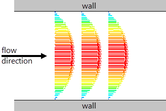
The wall shear stress vector.

A version of this field function is created for each phase in a multiphase continuum. This field function is volume fraction weighted for each phase.
Wall Shear Stress of <phase>
The wall shear stress vector for the specified phase. A version of this field function is created for each phase in a multiphase continuum.

This field function is volume fraction weighted for each phase.