Plotting Simulation and Experimental Data
Plot the lift and drag coefficients to determine when the analysis has reached convergence. The pressure coefficient on the wing is then compared against the experimental data [985]. In order to compare simulation results with experimental results, you create a normalized coordinate for a section of the wing.
-
To create a plot for drag coefficient:
-
To create a plot for the lift coefficient:
- Within the Reports node, copy and paste the Drag Coefficient report.
- Rename the copy to Lift Coefficient.
- Set the Direction property to [-sin(${AoA}), 0.0, cos(${AoA})].
- Right-click the Lift Coefficient node and select Create Monitor and Plot from Report.
Before plotting the pressure coefficient, create a unit to represent
the wingspan length.
-
To create the unit:
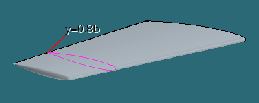
In the original experiments, flow data was measured along seven
sections in the spanwise direction. In this tutorial, you create a section plane at spanwise
location 0.8b (where b is the wingspan) and use this section for comparing computational and
experimental data. You also compare the pressure coefficient data.
-
To create a section plane at 0.8b:
-
Create two reports that calculate the minimum and maximum x coordinates on the wing,
respectively.
-
Create a field function that calculates the running distance (x) with respect to the
chord length (c) measured along the chord:
Use the field function to plot the numerical data for the pressure
coefficient.
-
To plot the numerical data:
- Right-click the Plots node and select .
- Rename the XY Plot 1 node to Pressure Coefficient.
- Select the Pressure Coefficient node and set Parts to
- Select the X Type node and set Data Type to Scalar.
- Select the and set x/c - y4 for the Field Function property.
- Select the and set Pressure Coefficient for the Field Function property.
-
To plot the experimental data:
- Right-click the node and select .
- Set Files of type: to (*.csv), then locate and open the file y=0.8b_experimental_data.csv.
- Right-click the node and select Add Data.
- In the Add Data Providers to Plot window, select y=0.8b_experimental_data and click OK.
The usual convention in aerodynamics problems is to reverse the y-axis orientation in pressure coefficient plots.
-
Select the node and set the following properties:
Property Setting Preferred X-Axis Left Axis Preferred Y-Axis Bottom Axis - Select the node and activate Reverse.
-
To set the correct titles for the plot:
- Select the node and set Title to Pressure Coefficient Comparison.
- Within , select the node and set Title to Distance (m).
- Select the node and set Title to Pressure Coefficient.
- Save the simulation.