Comparison With Experiment
Compare the results of the simulation with experimental data.
The main result of interest is the axial distribution of mean void. Since this result is a post processing calculation that is difficult to do without making a special assumption of a uniform grid, this calculation is made using a customized user macro:
- Select .
- In the Open dialog, navigate to your working directory and select wb_createAxialPlots.java.
-
Click
Open to run the macro.
The macro creates two new plots entitled Compare Axial Void and Compare Calorimetric Temperature. At the same time, the macro loads experimental data from file.
| Note | To refresh these plots, run the wb_deleteAxialPlots.java macro first. |
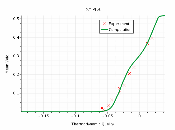
The Compare Axial Void plot is shown below:

The prediction of axial void is good near the start of net vapor generation and passes through the first few experimental points up to an intermediate level of void. Beyond this intermediate level, it over predicts the void by about 20% at the last experimental point. The agreement could be improved with model tuning. However, it is more satisfactory that this set of models and relaxation factors can provide solutions to many of the cases that are specified in Bartolemei (1982) [972] without any further adjustments.
This wide range of applicability is largely due to calibrations of Kocamustafaogulari and of Hibiki-Ishii to a wide range of pressures up to 150 bar. At 150 bar the bubble departure size becomes very small (about 5 micron compared to 50 micron for this test at 45 bar). It is also due to the capability of the S-gamma model to track the bubble size in subcooled flow starting from the Kocamustaogulari model for departure diameter.
For more information, see the following sections:
The Calorimetric Temperature that is provided by Bartolemei (1967) [971] is not fully explained in the paper, and is a little difficult to interpret. The name as translated from Russian suggests a velocity-weighted temperature averaged across the diameter, and the macro has prepared such an average from the computed results.
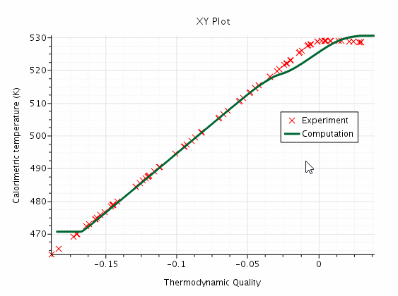
The Compare Calorimetric Temperature plot is shown below:

Bartolemei (1967) [971] does indeed provide a large number of points for Calorimetric Temperature as if these were experimental data. These points appear to lie on a straight line until a constant saturation temperature is reached exactly at zero thermodynamic quality.
The Simcenter STAR-CCM+ results deviate from this line when vapor is generated. This result is as expected from a heat balance, because if vapor coexists in subcooled conditions (thermodynamic quality < 0 ), liquid must be below the temperature that is expected for a homogeneous mixture.
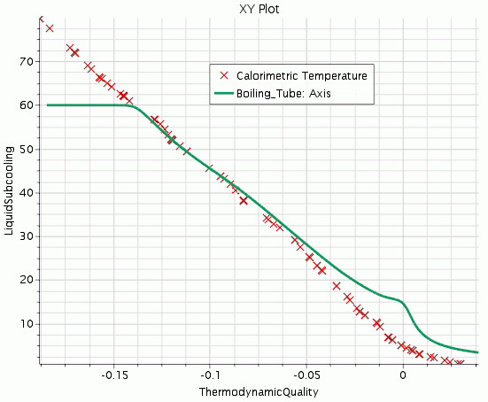
Now consider the liquid subcooling along the axis. The experimental data indicates that there was already a temperature gradient upstream of the heated section.
The source reference [Bartolemei (1967) [971]] gives no details here, but you are able to proceed by assuming that the simulation can model a short length of thermal boundary layer development before any boiling begins. This tutorial also uses the same thermodynamic quality scale to compare experiment and simulation, so that after some distance any differences due to inlet conditions become irrelevant.
The Axis Subcooling plot is shown below:

Here, as expected, the liquid subcooling is still above zero as the zero thermodynamic quality line is crossed. Heat is going into vapor production near the wall instead of heating the liquid core. The over prediction that Simcenter STAR-CCM+ makes of this core subcooling is consistent with its over prediction of outlet vapor.
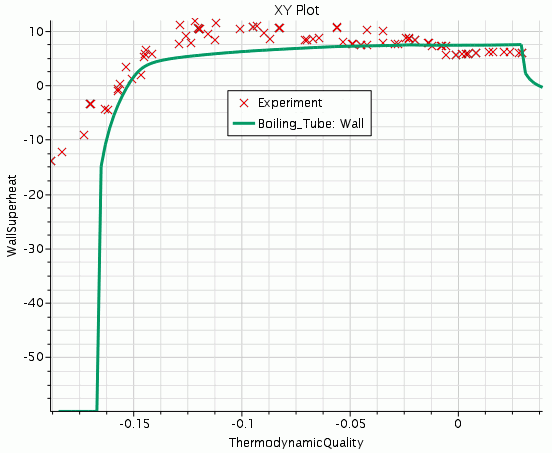
Finally compare the predicted and experimental wall superheat. Bartolemei (1967) [971] temperature measurements are used on the outside of the boiling tube, converted to inner face temperatures using Bartolemei’s own estimate of temperature drop in the tube wall.
The Wall Superheat plot is shown below:

It is clear that there was heating ahead of the specified heated section in the experiment, while Simcenter STAR-CCM+ takes a little distance to develop a thermal boundary layer. After this distance, the agreement is good at the start of boiling (zero superheat) and at fully developed boiling nearer the outlet where the superheat is of order 6K. In between, in the mixed convection/evaporation region, the current model underestimates superheat.
Again this model could be tuned to improve the superheat for this particular case (Bartolemei does not provide temperature data for any other conditions). However, it is good to see that this model could be useful for fixed-temperature applications as well as for fixed flux applications.