User-Defined Breakup Model

The User-Defined Breakup model lets you generate child parcels at secondary breakup events based on a breakup regime map you define. The breakup process is random, but properties like particle diameter are determined the same way for every droplet. The droplets do not have parent-child relationships after breakup events. This method is similar to the Stochastic Secondary Droplet (SSD) Breakup model.

Breakup regimes can be categorized in terms of several variables such as Weber number $W e$ or Ohnesorge number $O h$ , used in the breakup regime maps. The User-Defined Breakup model creates a map under each Breakup Regime Map node. Each breakup regime in the map corresponds to a breakup outcome. The following images show examples of breakup regime maps and breakup outcomes:

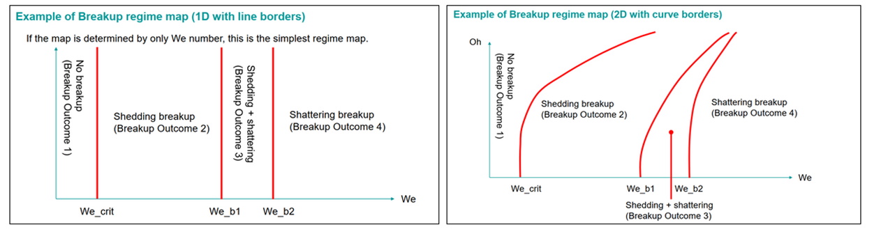
The left example is the simplest map which has only one independent variable (Weber number, We) to form the map. The right example has two axes, Weber number and the Ohnesorge number, and border lines between different breakup outcomes are not linear.

Breakup Onset Condition

For a given parcel to have a breakup event, it is necessary that the following conditions are satisfied:

The assigned breakup outcome is unequal to No Breakup.
Breakup growth time is greater than the breakup time-scale.

The breakup growth time is the accumulated parcel residence time while the parcel is assigned to any breakup outcome except No Breakup. Breakup growth time is reset to zero when the parcel has a breakup event.

Child Parcel Generation

The User-Defined Breakup model generates new child parcels from the parent parcel when the breakup onset criteria are satisfied. Then, the model defines diameter and velocity for both parent and child parcels. After the breakup, the parent-child relationship is irrelevant. The model determines the diameter for all droplets (parent and child parcels) from the size distribution function.

Child Droplet Size

The child droplet diameter is determined by the following methods:

Log-Normal Distribution

Droplet diameter

D

after breakup follows a log-normal distribution:

Figure 1. EQUATION_DISPLAY

F (D) = \frac{1}{2} (1 + e r f (\frac{\log (D / D_{0}) - m}{\sqrt{2} σ}))

(3119)

where:

$D_{0}$ is the parent droplet diameter.
$m$ is the mean value of $\log (D / D_{0})$ .
$σ$ is the standard deviation.

Root-Normal Distribution

Droplet diameters after breakup follow a root-normal distribution:

Figure 2. EQUATION_DISPLAY

F (D) = \frac{1}{2} (1 + e r f (\frac{\sqrt{D / D_{0}} - m}{\sqrt{2} σ}))

(3120)

Number of Child Droplets

The number of child droplets that are generated (including the parent droplet) is calculated as :

Figure 3. EQUATION_DISPLAY

N_{c} = min (N_{c}^{u}, N_{c}^{e})

(3121)

where

N_{c}^{u}

is the maximum number of child parcels and

N_{c}^{e}

is the smallest integer that satisfies the following condition:

Figure 4. EQUATION_DISPLAY

\sum_{c = 1}^{N_{c}^{e}} M_{c} \geq M_{p}

(3122)

where

M_{c}

is the mass of child parcel

c

and

M_{p}

is the mass of the parent parcel. Expressing the mass in terms of volume and density, the equation becomes:

Figure 5. EQUATION_DISPLAY

\sum_{c = 1}^{N_{c}^{e}} ρ_{c} \frac{π D_{c}^{3}}{6} n_{c} \geq ρ_{p} \frac{π D_{p}^{3}}{6} n_{p}

(3123)

where

D_{c}

and

D_{p}

are the diameters of the child and parent particles, and

n_{c}

and

n_{p}

are the child and particle counts.

n_{c}

is the value set in Target Count. The default for

n_{c}

is 1000.0.

Droplet Velocity After Breakup

The child droplet velocity is defined as:

Figure 6. EQUATION_DISPLAY

v_{c} = v_{p} + v_{t} n

(3124)

where:

$v_{c}$ is the velocity of the child particle.
$v_{p}$ is the velocity of the parent particle.
$v_{t}$ is the velocity magnitude of the child particle.
$n$ is the unit vector in the plane normal to $v_{p}$ , in a random direction

The default value is 0.