Running Unsteady with Curvature Correction
The accuracy of the simulation is improved by activating the curvature correction term of the k-omega turbulence model. However, this improved accuracy means that an unsteady solution must be adopted in order to achieve adequate convergence.
- Right-click the node and choose Select Models.
- Within the physics model selection dialog, make the following changes:
- From the Enabled group box, deactivate Steady.
- From the Time group box, activate Implicit Unsteady.
- Click Close.
- Select the node and set Curvature Correction to On.
Several changes are required for the solver settings and stopping criteria:
- Edit the Solvers node and set the following properties:
Node Property Value Implicit Unsteady Time-Step 5.0E-4 s Under-Relaxation Factor 0.9 Under-Relaxation Factor 0.4 - Edit the Stopping Criteria node and set the following properties:
Node Property Value Maximum Steps Enabled Deactivated Maximum Inner Iterations Maximum Inner Iterations 8 Maximum Physical Time Maximum Physical Time 0.5 s - Select the node and set Trigger to Time Step.
You can now run the solver again using the steady solution as the initial state:
- In the Solution toolbar, click
 (Run).The solver runs for another 8000 iterations (given 8 inner iterations per time-step).
 - Save the simulation. This action ensures that the simulation history file is complete.
- To compare the final solution from the unsteady run with the solution from the steady run:
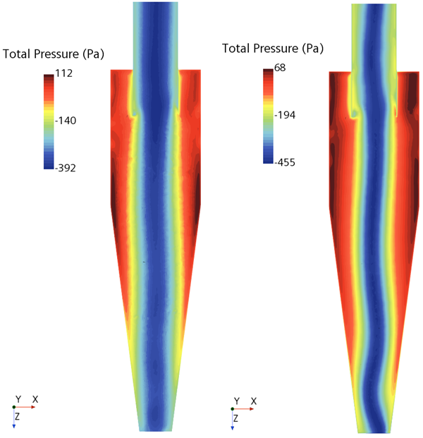
You can now compare the final unsteady solution on the right with the initial steady solution on the left. The addition of curvature correction has sharpened the center core of the swirling flow and defined its shape.