Validating the Results
Compare the results of the simulation with experimental data.
The computed temperature profile is validated by assuming that:
-
Saturation conditions are obtained after a distance of 1 m.
-
There are 6 K of superheat at the wall.
-
An analytical solution for axisymmetric heat conduction can represent the heat transfer across the fuel and cladding.
-
There is a contact resistance of 1.761E-4 (m2K/W) at the cladding-fuel interface.
-
The expected temperature at the center of the fuel is about 1000 C.
Import the expected radial temperature profile from a provided file:
- Right-click and select .
- In the Open dialog, navigate to the multiphaseFlow folder of the downloaded tutorial files, select the file WallBoilingCht.csv.
-
Click
Open to start the import.
The WallBoilingCht child node is created under Tables.
You create two derived parts that extract the radial temperature across the domain. Start with the fuel and cladding regions:
- Right-click Derived Parts and choose .
- Click the [Cladding, Coolant, Fuel] button in the Input Parts group-box.
- Deactivate the Coolant node, leaving Cladding and Fuel activated.
- Click OK.
-
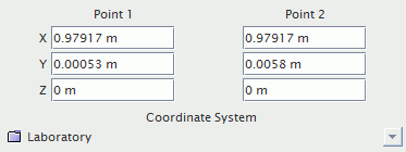
Enter the coordinates of
Point 1 and
Point 2 as shown:
- Leave the Coordinate System as Laboratory.
- Enter a Resolution of 5.
-
Select
No Displayer from the
Display group box.
The Create Line Probe window appears as shown.
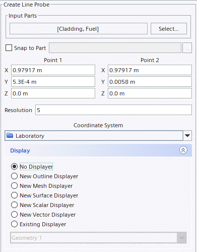
- Click Create, and then Close.
-
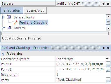
Rename
to
Fuel and Cladding.
To create a derived part for the coolant region, copy the Fuel and Cladding line probe and edit its properties:
- Right-click Fuel and Cladding and select Copy.
- Right-click Derived Parts and select Paste.
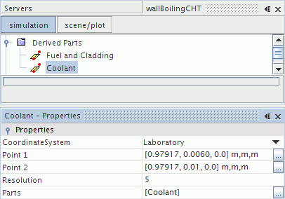
- Select the copy and rename it to Coolant.
- In the Properties window, set Point 1 to [0.97917, 0.0060, 0.0] m, m, m.
- Set Point 2 to [0.97917, 0.01, 0.0] m, m, m.
-
Click
 (Custom Editor) for the
Parts property.
(Custom Editor) for the
Parts property.
- In the Coolant - Parts dialog, right-click on a blank area and select Deselect All.
-
Activate
Coolant.
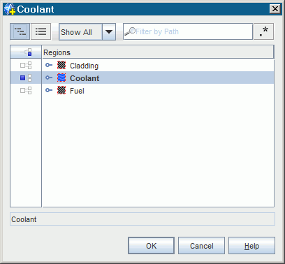
-
Click
OK.
The Coolant - Properties window appears as shown.
Create an X-Y plot that displays the radial temperature profile:
- Right-click Plots and select .
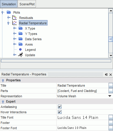
- Rename XY Plot 1 to Radial Temperature.
- In the Properties window, set its Title property to Radial Temperature.
-
Click
(Custom Editor) for the
Parts property.
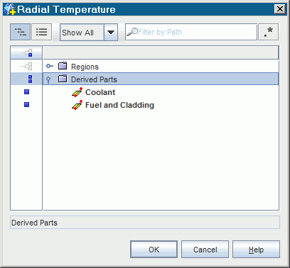
-
In the
Radial Temperature - Parts dialog, activate
Derived Parts.
Both Coolant and Fuel and Cladding parts are selected.
-
Click
OK.
- Select and set its Type property to Direction.
- Select and set its Value property to [0.0, 1.0, 0.0].
- Select and set its Field Function property to Temperature.
Create a second Y Type that displays the temperature in the coolant:
- Right-click and select New.
- Select and set its Field Function property to .
The temperature profile in the coolant is not plotted. Remove it from the display:
-
Select
and, in the
Properties window, deactivate
Lock Legend Name and then erase the
Legend Name.
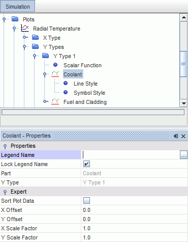
- Select and set its Shape to None.
- Select and, in the Properties window, deactivate Lock Legend Name and then erase the Legend Name.
- Select and set its Shape to None.
Import the expected profile as a table and add it to the plot:
- Right-click and select Add Data.
- In the Add Data Providers to Plot dialog, select WallBoilingCht and then click OK.
- Select the node and change the Legend Name to Expected Profile.
- Set the X Column to r.
- Set the Y Column to T.
- Select and set its Shape to None.
- Select the node.
- In the Properties window, set the Style to Solid.
-
Click
(Custom Editor) for the
Color property.
- In the Line Style - Colour dialog, click the Palette tab.
-
Select
Red.
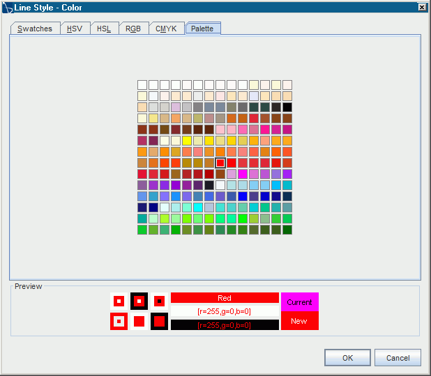
- Click OK.
- To add the X-axis title, select and, in the Properties window, set the Title to Position [0.0, 1.0, 0.0] (m).
-
To add the Y-axis title, select
and, in the
Properties window, set the
Title to
Temperature (K).
The Radial Temperature plot appears as shown.
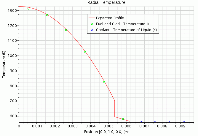
The computed temperature shows good agreement with the expected radial profile.
- Save the simulation.