Working with Monitor Plots

Monitor plots display the values collected by report-based and residual-based monitors as the solution is advanced. You can also use them to plot data from tables in the simulation.

For simulations that represent cyclic phenomena, such as for an internal combustion engine, you can activate Cyclic Mode in monitor plots and set the expected periodicity.

You can incorporate the data from a solution history into a monitor plot. See Retrieving Transient Solution Data.

Monitor plots can be renamed and deleted when they are no longer needed. Data from tables and data set functions may be plotted with the monitored data.

Use the following techniques:

Action

Instructions

Create a plot displaying the collected values of a monitor

Use one of the following techniques:

Right-click on the monitor node and select Create Plot from Monitor.

Note If more than one monitor is selected, then a plot is created based on the monitor that was selected first.
Right-click on the Plots node and select New Plot > Monitor and then add the desired monitors to the plot.

Normalize the values in a monitor plot

Use the Normalization Option of the monitor being plotted. See Normalizing the Monitor Data.

Plot the monitor of a report that addresses multiple parts

Set the Value Type property in the monitor node to Part Values. This option lets you monitor report values for some or all of the parts as well as the overall value. See Monitoring Report Results on a Per-Part Basis.

For cyclic simulations, apply periodicity to the monitor plot.

Select the monitor plot node and activate the Cyclic Mode property. This action makes two sub-nodes available:

Cyclic Settings
Data Series > [data set] > Cyclic Style

The monitor plot initially appears as a single cycle. See Cyclic Mode Properties Reference.

For cyclic simulations, display multiple cycles in a single display

Change the Period property to match the expected cycle length for the simulation.

For example, suppose your monitor plot has x-values of time from 0 to 1.0 seconds, and you want to display five cycles. Change the value of the Period property from 1.0 (equal to the full range of x-values) to 0.2. The plot shows five cycles, and the x-axis is limited to the new value of the period that you entered—that new value is repeated so that the total time of the cycles matches the original range of x-values.

Plot any monitor against any other

To add a monitor to the x-axis of the monitor plot, select the node of that plot and choose the monitor in the drop-down list of the x-Axis Monitor property.

About this Feature

In a default monitor plot, the y-axis uses any one of various monitors while the x-axis represents solution progress. (The x-axis uses the Iteration monitor in a steady simulation and the Physical Time monitor in an unsteady one.)

However, the added flexibility of plotting monitors against one another helps you determine correlations between monitors, especially over time. As the simulation run progresses, some monitors define non-monotonic functions: periodic ones such as crank angle, and oscillating ones such as wave height.

Each monitor has an independent data sampling policy based on its Trigger and Frequency properties. It is not guaranteed that the x- and y-axis monitors sample data at the same rate. Therefore, while the y-axis monitor collects a sample at a given iteration, the plot does not update until the x-axis monitor has also collected a sample.

Note

The Trigger property of a monitor does not control the frequency at which the data is plotted. It specifies the frequency at which the monitor collects the data. To control the frequency at which the data is queried and plotted, use the Update feature of the plot node itself. If you want to plot data against physical time, make sure that the same Physical Time monitor exists throughout the solution. Otherwise the plot data appears incomplete. If you are running a steady solution but expect to need a plot with physical time, start by running the unsteady solver then switch to the steady one; this ensures that Physical Time exists in the simulation.

Create a custom residual plot

Create a monitor plot.
Add the residual monitors of your choice to the plot.

Display computation errors in a monitor plot

Select the node of the monitor data set for which you want to view the errors.
Activate the Show Warning Symbol property.

Error data points are visually differentiated and the plot legend displays this differentiation for the report monitor's data series legend.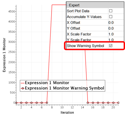

Interactive runs show errors when they occur.

Monitor plots will have a state history for batch runs for subsequent review.

Edit the colors of the cyclical plot

Right-click the Data Series > [data set] > Cyclic Style node and select Edit Child Colors. In the Data Provider Colors dialog, edit colors associated with cycle lines.

The Pitch of a Boat

This example uses an unsteady case from a tutorial simulating the motion of a boat in head waves. The purpose is to show a correlation analysis between different monitored variables, in this example y-rotation against z-translation:

Right-click the monitor node (Z Translation Monitor in this example) and select Create Plot from Monitor.

Note	It is possible to set up a monitor plot using two other techniques: creating an empty monitor plot node and adding the monitors manually, or creating a monitor plot simultaneously with a report-based monitor.

By default this plot has the following characteristics:
- The title of the plot has the name of the monitor.
- The monitor that was used to create this plot is selected for the y-axis.
- The x-axis is Physical Time because this case is unsteady. (In a steady case, the x-axis would be Iteration.)
To reflect the content of the plot, change the Title property of the plot node. In this example, the new name is BoatInHeadWaves (Y Rotation and Z Translation).
To add a monitor to the x-axis of the monitor plot, select the node of that plot and choose the monitor in the drop-down list of the x-Axis Monitor property. (In this example it is the Y Rotation Monitor.)

The resulting plot is shown in the following screenshot.