Chemical Kinetics

When modeling reacting species transport, providing a source term to the transport equations requires calculation of the reaction rates (chemical kinetics) for all reactions in the chemical mechanism.

Reaction Rate

The reaction rate for elementary reactions is calculated as follows.

there are two reactant species and one product species. In order for the reaction to proceed, the reactant molecules must collide with energy that is equal to or greater than the activation energy $E_a$ . The rate $r_k$ at which this overall reaction proceeds is also dependant upon the rate constant $k$ , and for an elementary reaction, the concentration of the two reactants to the power of their stoichiometric coefficients.

The chemical formula of a species in square brackets represents the concentration of that species in the reaction mixture.

The production (or consumption) rate $r_i$ of species $i$ , depends on the reaction rates of the reactions which produce and consume the species, and on the concentration of all species which participate in those reactions. The total net rate is therefore a sum of Eqn. (3360) over all reactions in which species $i$ participates. In the equation below, $j$ (=1, 2, … , $N_j$ ) denotes reactions and $i$ denotes species.

The net reaction rate of species i, denoted ${\dot{\omega }}_i$ , is the sum over all reactions ( $r_j$ in Eqn. (3358)) multiplied by the stoichiometric coefficient.

where the rate coefficients, $k_f$ for the forwards reaction and $k_b$ for the backwards reaction, are determined by Eqn. (3365).

The user-defined reaction rate is calculated from:

Rate Constant

Chemical Heat Release Rate

The chemical heat release rate is defined as:

where ${\dot{\omega }}_k$ is the net reaction rate of the $k\prime th$ species, and $h_k^o$ is the formation enthalpy of the $k\prime th$ species. When using the Species Transport models, Eqn. (3366) is evaluated and available as a field function named Chemical Heat Release Rate.

For the Flamelet Generated Manifold (FGM), and partially premixed Chemical Equilibrium (CE) and Steady Laminar Flamelet (SLF) models, the chemical heat release rate is calculated as:

where $\dot{c}$ is the progress variable source term, and $h_R$ is the heat of reaction. $h_R$ is calculated assuming the fuel is a hydro-carbon reacting with oxygen in a 1-step reaction as:

The heat of reaction is calculated as:

where $Y_k^F$ is the mass fraction of the $k\prime th$ species in the fuel stream.

For non-premixed SLF, the chemical heat release rate is calculated as:

where $\chi$ is the scalar dissipation rate.

Note that the chemical heat release rates for flamelet models are an approximation of the exact heat release rate from Eqn. (3366), and the field function is named Chemical Heat Release Rate Indicator.

Third Body Reactions

Third Body Efficiencies

Some reactions require a “third body” in order to proceed, as in:

$$H+O_2+M\leftrightarrow H{O}_2+M$$

(3371)

where $M$ represents the third body. Third bodies act as a form of catalyst. Typically, any species in the mixture can act as a third body. Third bodies affect the rate at which the reaction proceeds.

The expression for the reaction rate for a reaction which requires a third body is as follows:

$$r_j=\left(\underset{i=1}{\overset{N}{\mathrm{\Sigma }}}\right({\alpha }_{ij}\left)\right[X_i\left]\right)(k_{f,j}\underset{i=1}{\overset{N}{\mathrm{\Pi }}}{\left[X_i\right]}^{{\upsilon }_{ij}^{\prime }}-k_{b,j}\underset{i=1}{\overset{N}{\mathrm{\Pi }}}{\left[X_i\right]}^{{\upsilon }_{ij}^{\prime \prime }})$$

(3372)

for species $(i=1,\mathrm{...},N)$ :

• ${\alpha }_{ij}$ represents the collision efficiency of the third body
• $k_{f,j}$ is the forward rate constant of reaction $j$
• $k_{b,j}$ is the backwards rate constant of reaction of reaction $j$

When ${\alpha }_{ij}=1$ , all species in the mixture contribute equally as third bodies and the total concentration of the mixture is:

$$\left[M\right]=\underset{i=1}{\overset{N}{\mathrm{\Sigma }}}\left[X_i\right]$$

(3373)

However, when ${\alpha }_{ij}\ne 1$ , the concentration of the effective third body in the reaction is:

$$\left[M\right]=\underset{i=1}{\overset{N}{\mathrm{\Sigma }}}\left({\alpha }_{ij}\right)\left[X_i\right]$$

(3374)

where ${\alpha }_{ij}$ is specified for the third body species in the reaction mechanism.

Pressure-Dependent Chemical Reaction Rates

Pressure dependent chemical reactions (fall-off reactions) have a first-order rate at low pressure and become zero-order as the concentration of the third-body species increases. In this type of reaction, the rate is affected by pressure as well as temperature, Simcenter STAR-CCM+ calculates the rate constants using the pre-exponential factor $A$ that is provided by the reaction mechanism:

$$k=k_{\infty }\left(\frac{P_r}{1+P_r}\right)F$$

(3375)

where the reduced pressure $P_r$ is,

$$P_r=\frac{k_0\left[M\right]}{k_{\infty }}$$

(3376)

where $\left[M\right]$ is the concentration of the species $M$ with third-body efficiencies.

The low pressure limit $k_0$ is,

$$k_0=A_0{T}^{\beta 0}\exp (-\frac{E_0}{R_{u}T})$$

(3377)

and the high pressure limit $k_{\infty }$ is,

$$k_{\infty }=A_{\infty }{T}^{\beta \infty }\exp (-\frac{E_{\infty }}{R_{u}T})$$

(3378)

The blending (fall off) function, $F$ , is calculated differently, depending on the approach that you use to specify the pressure-dependent parameters.

• Using the Lindemann method, $F$ is calculated as unity, $F=1$
• Using the Troe method, $F$ is calculated as:

  $$\log F={[1+{\left[\frac{\log P_r+c}{n-d(\log P_r+c)}\right]}^2]}^{-1}\log F_{cent}$$

  (3379)
  where:

  $$F_{cent}=(1-\alpha )\exp (-\frac{T}{T^{***}})+\alpha \exp (-\frac{T}{T^{*}})+\exp (-\frac{T^{**}}{T})$$

  (3380)

  • $c=-0.4-0.67\log F_{cent}$
  • $n=0.75-1.27\log F_{cent}$
  • $d=0.14$
  • $\alpha$ , $T^{***}$ , $T^{*}$ , and $T^{**}$ are constants that you specify within the imported chemical mechanism
• Using the (SRI) method, $F$ is calculated as:

  $$F=d{[a\exp (\frac{-b}{T})+\exp (\frac{-T}{c}\left)\right]}^X{T}^e$$

  (3381)
  where a, b, c, d, and e are parameters that you specify within the imported chemical mechanism. When d and e are not specified in the mechanism, they are set to 1 and 0 respectively, by default.

  $$X=\frac{1}{1+{\log }^2{P}_r}$$

  (3382)

For both the Troe and SRI methods, $F$ approaches unity for both high and low pressure limits.

Chemically-Activated Bimolecular Reaction Rates

Pressure Dependence Through Logarithmic Interpolation (PLOG)

When using the PLOG method to describe the pressure dependence of a reaction rate, the reaction rate is calculated by the Arrhenius expression Eqn. (3365) using rate parameters ( $\beta$ , $E_a$ , and $A$ ) that are modified for different pressures.

Rate parameters are given for a discrete set of (at least two) different pressures within the pressure range of interest.

Chemical Equilibrium

When the forwards and backwards reaction rates are equal, the reaction is said to have reached equilibrium and no net reaction is observed. The proportions of reactants and products are constant as long as the pressure (for gas-phase reactions), temperature, and concentrations of species are constant.

You can determine the amount of each species that is present at equilibrium using the equilibrium constant, $K$ .

where $c^0$ is a reference concentration.

Surface Chemistry

For example, in the diagram below, a gas molecule is adsorbed onto a surface next to a previously adsorbed surface species. The gas molecule is broken up into its constituent atoms. Some of the adsorbed atoms react to form smaller gas molecules which leave the surface. One atom from the gas molecule remains adsorbed as a surface species, and the previously adsorbed surface species becomes a bulk species.

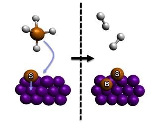
The reaction in the diagram above can be represented by:

Bulk species are not considered reactive but can end up on a surface site if the surface molecules previously covering the bulk species are desorbed or take part in a reaction.

The general surface reaction form for reaction $j$ is:

where:

• $G_i$ , $S_i$ , and $B_i$ are gas, site, and bulk species.
• $N_g$ , $N_s$ , and $N_b$ are the numbers of gas, site, and bulk species.
• ${\mathrm{g\prime }}_{i,j}$ , ${\mathrm{s\prime }}_{i,j}$ , and ${\mathrm{b\prime }}_{i,j}$ are stoichiometry coefficients for gas, site, and bulk reactants.
• $g_{i,j\prime \prime }$ , $s_{i,j\prime \prime }$ , and $b_{i,j\prime \prime }$ are stoichiometry coefficients for gas, site, and bulk products.

The rate of the $j$ th reaction is then:

where $p_g$ and $p_s$ are rate exponents for reactants, and ${\left[\text{*}\right]}_{\text{wall}}$ represents molar concentration on the wall. The forward rate constant $k_{f,j}$ for reaction $j$ is given by an Arrhenius expression. Which, for the simplest type of the reaction, is given by Eqn. (3365) (where $k$ is $k_{f,j}$ ).

The sum runs over all different site types.

It is assumed that the reaction rate does not depend on the concentrations of the bulk species.

The net molar rate of change per surface area (production or consumption) of each species $i$ is given by:

For some surface reactions, the reaction rate is influenced by the surface coverage characteristics of the species that are involved. The arrhenius rate expression, Eqn. (3365), can be modified to create a corrected rate constant as follows:

Particle Chemistry

For reactions of particles, the rate constant $k$ is determined using the Arrhenius equation Eqn. (3365). Since particle chemistry reaction rates consider diffusion alongside kinetics, these calculations are described in the Particle Reactions section of the Theory Guide.