Setting the Initial Conditions
You set the initial conditions for the physics continuum.
A field function sets up the initial pressure field as a linear profile: this profile is close to the expected solution. Setting the initial pressure in this way reduces the time that is required to obtain a solution. The pressure profiles at the inlet and outlet are specified to define the linear pressure field correctly.
In this case, the inlet is not modeled as a velocity inlet, since the simulation diverges when the whole-cross section is frozen, and the flow stops. A combination of pressure outlets at both inlet and outlet allows the flow to be stopped completely in the duct without violating any boundary condition
When choosing initial conditions, it is important to select a field that is bounded by the boundary conditions to avoid divergence. To satisfy this criterion, specify a linear pressure field with maximum and minimum values that are set as the boundary conditions.
The initial temperature is set to the inlet temperature. The initial velocity field is set to be close to the expected average velocity during the initial stages of the flow, that is, before the freezing commences, for faster convergence.
To set the initial conditions:
-
Create the following field functions using the same procedure as in the
previous section.
The desired gauge inlet pressure is taken as 1.0 Pa.
Node Title
Target Inlet Pressure
Dimensions
Pressure
Function Name
TargetInletPressure
Definition
1.0
As previously mentioned, the inlet is modeled as a pressure outlet: the dynamic pressure and turbulent stresses are added to make sure that the static inlet pressure is always 1.0 Pa.
Node Title
Inlet Pressure
Dimensions
Pressure
Function Name
InletPressure
Definition
${TargetInletPressure} + 0.5*${Density}*pow(mag($${Velocity}), 2)
The outlet pressure is set to 0.0 Pa.
Node Title
Outlet Pressure
Dimensions
Pressure
Function Name
OutletPressure
Definition
0.0
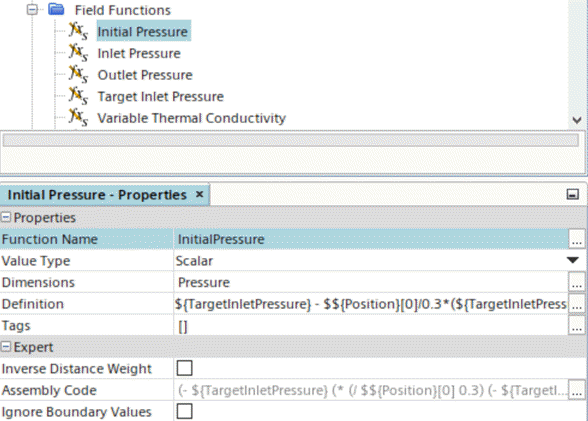
The initial pressure field is then taken as a linear profile from 1.0 Pa at X = 0 m to 0.0 Pa at X = 0.3 m at the lower end of the pipe.
Node Title
Initial Pressure
Dimensions
Pressure
Function Name
InitialPressure
Definition
${TargetInletPressure} - $${Position}[0]/0.3*(${TargetInletPressure} - ${OutletPressure})
-
Right-click and select Refresh to order the created
field functions alphabetically.
-
Edit the
node and set the following properties:
Node Property Setting Pressure Method Field Function Scalar Function Initial Pressure Static Temperature Value 273.1 K Velocity Value [0.012, 0.0] m/s Volume Fraction Value [1.0] 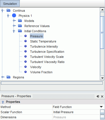
- Save the simulation.