Anisotropic Meshing for Lifting Surfaces
Anisotropic meshing allows you to generate a surface mesh that contains stretched quad elements aligned with features (anisotropic faces). By using stretched elements, you can reduce the number of faces in the mesh while retaining geometrical and solution accuracy.
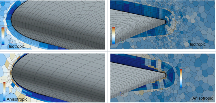
When meshing aerospace geometries such as wings, propeller blades, or turbine blades, you are required to generate a fine mesh that adequately captures the curvature of the leading and trailing edges. In general, you want the mesh to be aligned to the leading and trailing edges and to be stretched in the spanwise direction (with short edges in the streamwise direction). To help reduce the cell count while maintaining solution accuracy, you can apply anisotropic meshing to these edges. It is computationally less expensive to use anisotropic mesh in comparison to isotropic.
In order to use the anisotropic meshing option, your volume mesh must be based on an initial quadrilateral surface mesh. Before using anisotropic meshing, make sure that you have part curves along the leading and trailing edges of the wing, and that the starting geometry represents the fluid.
- Right-click the node and select .
-
In the Create Automated Mesh Operation
dialog:
- Select the node and set Meshing Method to Quad Dominant.
- Expand the node and set the parameters that you require for the overall fluid domain.
- Right-click the node and select .
-
Select the Curve Control node and in the Properties window:
- Select the node and activate Specify anisotropic surface size settings.
-
Under the Values node, set the Growth
Ratio, Maximum Aspect Ratio, Number of Constant
Layers, and First Layer Thickness to values
that suit your scenario.
For more information, see Curve Controls and Values.
-
To generate a good quality mesh where two opposite part curves are connected
together in a cusp:
- Select the node and activate Specify anisotropic mesh distribution between close Part Curves.
- Under the Values node, set the Minimum Layer Size in Narrow Regions of Thin Areas and the Minimum Number of Layers to values that suit your scenario.
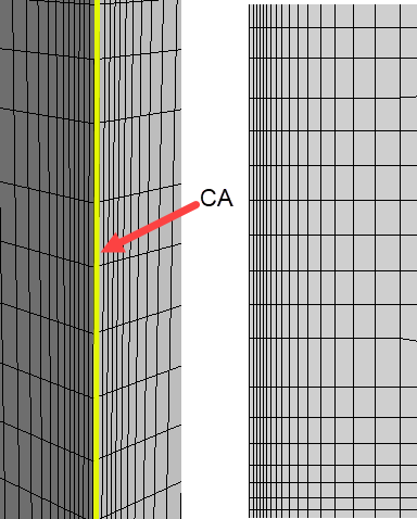
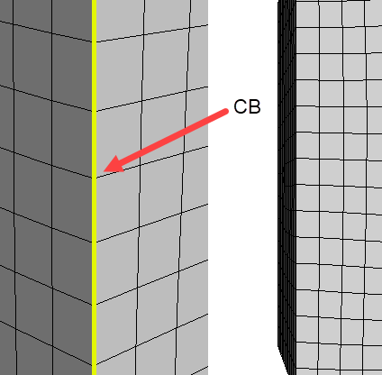
For more information, see Curve Controls and Values.The image below shows two examples with the same First Layer Thickness value. The first example on the left displays a mesh where the Specify anisotropic mesh distribution between close Part Curves option is deactivated. The second example on the right shows a mesh where the option is activated and the Minimum Number of Layers is set to 3 and the Minimum Layer Size in Narrow Regions of Thin Areas value is set to a small value.
Anisotropic boundary layers grow from the part curve as long as the first layer thickness is smaller than the target size of the surface in that specific location. The target size for the surface determines the width of cell faces along the length of the part curve. Hence, by choosing the target size and first layer thickness correctly, you can achieve the stretched faces along the spanwise direction. For cases where the target size is smaller than the anisotropic first layer thickness, the mesh does not generate any anisotropic boundary layer.
When anisotropic meshing is enabled on a curve, the surface remesher generates a number of face layers (n) of fixed size, normal to the curve. Starting from n+1, the anisotropic layers grow in size with a ratio equal to the growth ratio until the anisotropic size of the layers are the same as the isotropic size (target size) of the surface in that position.
- Execute the Automated Mesh Operation.
- Create a scene to visualize the mesh. See Mesh Visualization.