Setting Up Body Constraints
Simcenter STAR-CCM+ supports three constraint types—Contact Constraint, Velocity Driver, and Distance Driver for 3D bodies with Multi-Body Motion option.
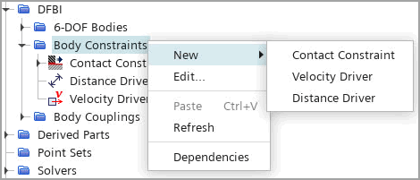
- To define a body constraint:
-
Right-click and select .
The available body constraint types are:
- To verify the correctness of the constraint solution during the simulation, plot the 6-DOF Constraint Deviation Report. It calculates the maximum normalized deviation from the constraint equations. Typically, this report value should be below 1e-3:

If the constraint deviation that you monitor is too large, , refer to the guidelines in Setting Up Multi-Body Motion.
See also: 6-DOF Constraint Deviation.
-
Right-click and select .
- To define the edge and the orientation of the sliding plane, you can specify the Origin, Direction, and Normal vectors in the laboratory coordinate system. You can also create a new coordinate system where the origin is at the edge of the plane and one axis points in the direction of the plane:
- (Optional) To model the friction force on the sliding surface, select the node and set the Dynamic Friction Coefficient and Static Friction Coefficient.

For more details, refer to [contact constraint] Properties. - (Optional) To model the friction force on the sliding surface, select the node and set the Dynamic Friction Coefficient and Static Friction Coefficient.
- To prescribe the velocity of a 6-DOF body using an absolute value, you define the velocity of the body relative to the environment. To do this:
- Set Velocity to a constant value.
In the following setup,the center of mass of Body 1 moves at a speed of 0.1m/s in the x direction of the Laboratory coordinate system:

- Set Velocity to a constant value.
The Velocity and Direction specified in the velocity driver must be consistent with the initial velocity and angular velocity of all the participating bodies. In this example, you set the initial velocity of the body to [0.1, 0, 0] m/s in the laboratory coordinate system. To make sure the settings are consistent, you can use the InitialVelocityOfDfbiConstraint field function. Use this field function in the Velocity property of the velocity driver.
-
To specify velocity as a function of time, you can use the field function in an
expression, such as
${InitialVelocityOfDfbiConstraint1}*cos(2.0*acos(-1.0)*${Time}).

At t=0, the expression evaluates to the InitialVelocityOfDfbiConstraint 1 field function, so that the velocity driver is consistent with the initial velocity of the 6-DOF body.
-
A relative velocity driver specifies a relative velocity between two 6-DOF
bodies.
The following example demonstrates the velocity of Body 1 center of mass relative to the Body 2 center of mass, in the x direction of the Body 1 coordinate system:

-
For two bodies initially at rest, you create a dynamical Distance Driver and
specify the Distance between the
bodies as a sinusoidal function of time —
${InitialDistanceOfDfbiConstraint3}+
0.1*sin(4.0*${Time}).
At t=0, although the initial distance is consistent with the body initial conditions (using the ${InitialDistanceOfDfbiConstraint3} built-in field function), the time derivative, and therefore, the initial velocity, is non-zero, so it is not consistent with the body initial velocity.
To resolve this inconsistency, you can change the initial velocities of the bodies and/or the time-dependence of the Distance definition, which can require very complicated calculations. In many cases, it is convenient to introduce a blending time of, for example, 0.5s, which defines a time window during which the body initial conditions are blended automatically into the user-specified distance. During the blending time, the distance applied by the Distance Driver changes to be consistent with the body initial conditions, and after the blending time the distance matches the user-defined distance.
To set a blending time, select the node and specify Blending Time.

