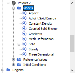
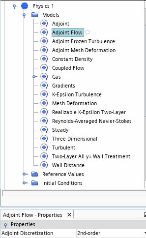
An adjoint analysis is performed in two major steps. First, you simulate the steady problem using the coupled flow model, or both the coupled flow and coupled energy models. The result of this simulation is referred to as the "primal solution". The primal solution can involve isothermal fluid flow, fluid flow with energy, conduction in solids, or conjugate heat transfer between fluids and solids. In a following step, you set up and run the adjoint analysis starting from the previously obtained primal solution. Instead of running an adjoint simulation stepwise, Simcenter STAR-CCM+ also provides the methodology to set up a user defined adjoint workflow through Simulation Operations.
The robustness of the adjoint solution relies heavily on the fidelity of the primal flow and energy field. This dependency means that the primal solution must have a good convergence. Usually a reduction of 5 orders of magnitude in the continuity residual is sufficient. To enhance the convergence of the primal solution, create a mesh of good quality before you start the simulation.
You are advised to use a double precision version of Simcenter STAR-CCM+ for the simulation.
To set up an adjoint analysis:
- Create a suitable, high-quality volume mesh.
Check the mesh quality and improve it if necessary.
For more information, see Checking the Volume Mesh
One measure that is useful for improving the quality of polyhedral meshes is the mesh optimizer. To improve the quality of a polyhedral mesh, increase the number of optimization cycles and increase the quality threshold. The mesh optimization leads to a longer meshing time.
For more information, see Volume Mesher Controls and Values
- Set up a steady-state flow and/or a heat transfer analysis using models and features compatible with the adjoint solver.
- To set up a coupled flow analysis, for the fluid physics continuum, select the following physics models:
| Group Box | Model |
|---|
| Space | Two Dimensional or Three Dimensional |
| Time | Steady |
| Material | Gas or Liquid |
| Flow | Coupled Flow |
| Equation of State | - Constant Density
- Ideal Gas
or |
| Viscous Regime | |
| Optional Models | (optional) Passive Scalar In cases where you track the concentration of passive scalars, including those with user-defined source terms, you can use passive scalars in reports that you later assign to adjoint cost functions. Adaptive Mesh—Use this model if you want to refine the mesh locally and select user-defined refinement criteria that query the flow solution as the simulation runs to control solution fidelity. Select the User-Defined Mesh Adaption criteria and specify the appropriate properties. |
- To set up a coupled solid energy analysis compatible with adjoint, for the solid physics continuum, select the following physics models:
| Group Box | Model |
|---|
| Space | Two Dimensional or Three Dimensional |
| Time | Steady |
| Material | Solid |
| Optional Models | Coupled Solid Energy |
| Equation of State | Constant Density |
- Run the simulation until it converges.
- If you are running a flow solution, select the adjoint flow model:
- Right-click the node and select Select models...
- In the Physics Model Selection dialog, select Adjoint from the Optional Models group box.
The Adjoint Flow model is automatically selected.
- From the Adjoint Turbulence group box, select the option that corresponds with the turbulence model for the primal flow, if one was selected. The options are as follows:
| Viscous Regime | Reynolds-Averaged Turbulence | Adjoint Turbulence |
|---|
| Inviscid | - | Not Applicable |
| Laminar | - | Not Applicable |
| Turbulent | K-Epsilon Turbulence | Adjoint Frozen Turbulence |
| Turbulent | K-Omega Turbulence | Adjoint Frozen Turbulence |
| Turbulent | Reynolds Stress Turbulence | Adjoint Frozen Turbulence |
| Turbulent | Spalart-Allmaras Turbulence | - Adjoint Frozen Turbulence
- Adjoint Spalart-Allmaras
|
- After specifying the Adjoint Turbulence model, select additional models regarding the simulation purpose:
| Optional Adjoint Models | Application |
|---|
| Adjoint Mesh Deformation | Computes the field function Adjoint of [cost function] w.r.t Position. Select this model when you run a shape optimization using deformation field based on the mesh sensitivity on control points. This model requires Mesh Deformation from the Optional Models group box. See also: Computing the Mesh Sensitivity |
| Surface Sensitivity | Computes the field function Surface Sensitivity of [cost function] w.r.t Position. Select this model when you run a shape optimization using deformation field based on the surface sensitivity on boundaries. If you run a surface sensitivity analysis without performing a shape optimization. This model doesn't require any extra model. In case of a shape optimization, it requires Mesh Deformation from the Optional Models group box. See also: Computing the Surface Sensitivity |
| Topology Optimization | Select this model when you run an adjoint-based topology optimization. This model activates automatically the Topology Physics model. It doesn't require any Optional Models . See also: Adjoint Topology Optimization |
| Adjoint Passive Scalar | Select this model when you want to perform an optimization related to the advection of a quantity that you track using a passive scalar. For example, when determining the sensitivity of the concentration of a passive scalar at an outlet with respect to the shape of a duct in which the scalar is injected. |
- Click Close.
- For the adjoint flow model, set the discretization scheme:
| Adjoint Discretization | The discretization scheme that is used for the adjoint flow model. |
| 2nd-order | This setting is the default. Use the second order discretization scheme for best accuracy of the adjoint solution. |
| 1st-order | Use the first order discretization scheme in the event the adjoint solver does not converge with the default second order setting. This setting makes the adjoint solver less accurate but more robust. |
- If you activated the Adjoint Passive Scalar model, select the model node and set its properties as follows:
- Set Passive Scalars to those passive scalars for which you want to compute the adjoint.
- Set Secondary Gradients and Convection to match the settings used for the Passive Scalar model in the primal flow. In the case of convergence issues with the adjoint, you can try reducing model accuracy in the adjoint solution, for example by deactivating secondary gradients.
- If you are running a heat conduction analysis in solids, select the adjoint solid energy model:
- For the solid physics continuum, , select Adjoint from the Optional Models group box.
The Adjoint Solid Energy is automatically selected if Coupled Solid Energy is enabled. The Mesh Deformation model is automatically selected.

- To create one or more adjoint cost functions, refer to Creating the Adjoint Cost Functions.
- To define the adjoint solver stopping criteria, refer to Defining Adjoint Stopping Criteria.
- Set up and run the adjoint solver. Refer to Running the Adjoint Solver.
- To compute the surface sensitivity, select the Surface Sensitivity model from the Optional Models group box. Through the surface sensitivity you can quickly assess which areas in the geometry are most critical to the cost functions of interest. For more details, refer to Computing the Surface Sensitivity.
- To compute the impact of the boundary condition parameters on the cost functions of interest, refer to Computing Adjoint Parameter Sensitivity.
- To highlight the locations where the numerical inaccuracy impacts the accuracy of cost function, refer to Computing Adjoint Error Estimates.
- To visualize the results using the adjoint field functions, refer to Visualizing the Adjoint Solution and Visualizing the Mesh Sensitivity.
- To set up a shape optimization, refer to Adjoint Shape Optimization Workflow.
- To set up a topology optimization, refer to General Workflow for Adjoint Topology Optimization.
For a complete workflow using Adjoint, refer to the following tutorials:

